CS224W-Machine Learning with Graph-Fast Neural Subgraph
Subgraphs and Motifs
Definition:
- Given graph :
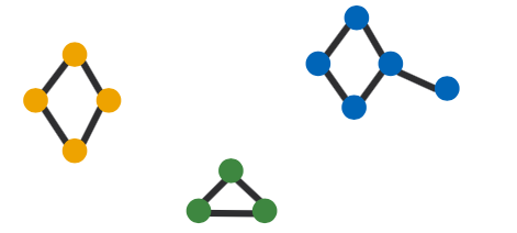
- Def 1. Node-induced subgraph: Take subset of the nodes and all edges induced by the nodes:
- is a node induced subgraph iff
-
-
- is the subgraph of induced by
Alternate terminology: “induced subgraph”
- is a node induced subgraph iff
- Def 2. Edge-induced subgraph: Take subset of the edges and all corresponding nodes
- is an edge induced subgraph iff
-
-
Alternate terminology: “non-induced subgraph” or just “subgraph”
- is an edge induced subgraph iff
- Def 1. Node-induced subgraph: Take subset of the nodes and all edges induced by the nodes:
The best definition depends on the domain!
- Example:
- Chemistry: Node-induced (functional groups)
- Knowledge graphs: Often edge-induced (focus is on edges representing logical relations)
The preceding definitions define subgraphs when and , i.e. nodes and edges are taken from the original graph .
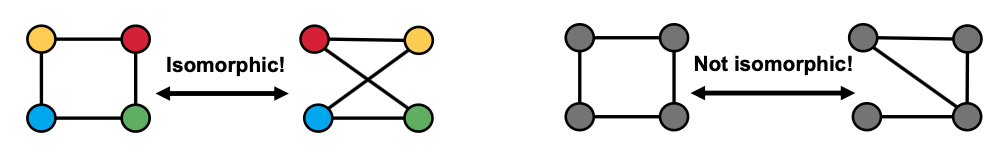
Graph Isomorphism
Graph isomorphism problem: Check whether two graphs are identical:
- and are isomorphic if there exists a bijection such that iff
- is called the isomorphism
We do not know if graph isomorphism is NP-hard, nor is any polynomial algorithm found for solving graph isomorphism.
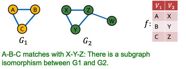
- is subgraph-isomorphic to if some subgraph of is isomorphic to
- We also commonly say is a subgraph of
- We can use either the node-induced or edge-induced definition of subgraph
- This problem is NP-hard
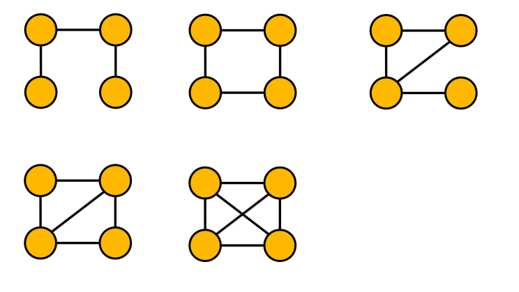
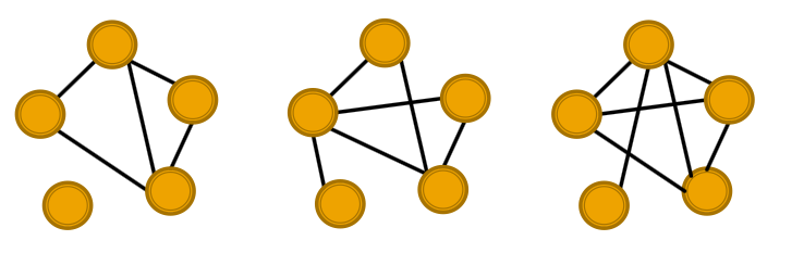
- Case Example of Subgraphs
- All non-isomorphic, connected, undirected graphs of size 4
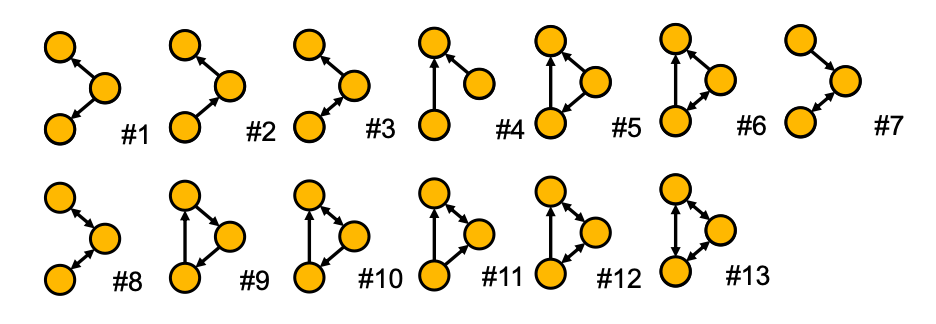
- All non-isomorphic, connected, directed graphs of size 3
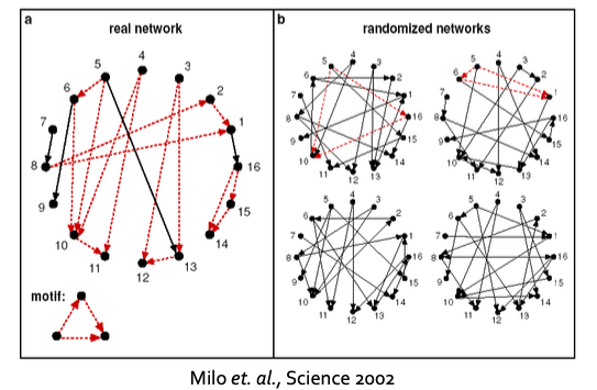
Network Motifs
- Network motifs: “recurring, significant patterns of interconnections”
- How to define a network motif:
- Pattern: Small (node-induced) subgraph
- Recurring: Found many times, i.e., with high frequency. How to define frequency?
- Significant: More frequent than expected, i.e., in
Motifs: Induced Subgraphs
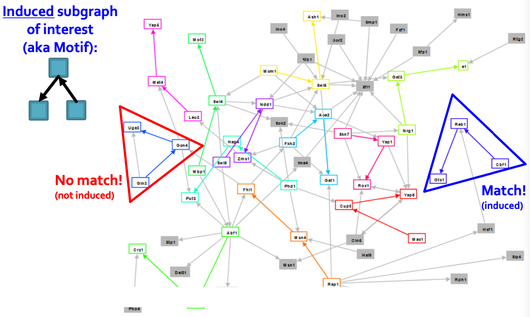
the red region has 3 edges.
Why do we need motifs?
- Motifs:
- Help us understand how graphs work
- Help us make predictions based on presence or lack of presence in a graph dataset.
- Example:
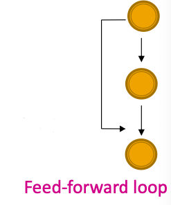
- Feed-forward loops: Found in networks of neurons, where they neutralize “biological noise”
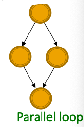
- Parallel loops: Found in food webs
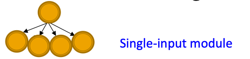
- Single-input modules: Found in gene control networks
Subgraphs Frequency
- Let be a small graph and be a target graph dataset.
- Graph-level Subgraph Frequency Definition
Frequency of in : number of unique subsets of nodes of for which the subgraph of induced by the nodes is isomorphic to
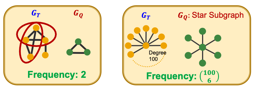
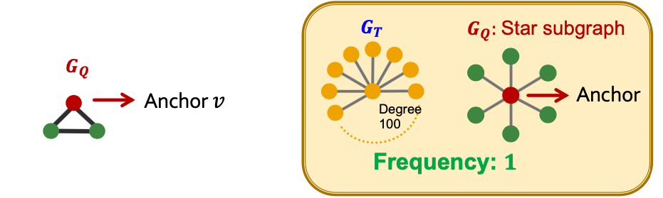
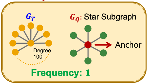
- Let be a small graph, be a node in (the “anchor”) and be a target graph dataset.
- Node-level Subgraph Frequency Definition: The number of nodes in for which some subgraph of is isomorphic to and the isomorphism maps node to .
- Let be called a node-anchored subgraph
- Robust to outliers
What if the dataset contains multiple graphs, and we want to compute frequency of subgraphs in the dataset?
- Solution: Treat the dataset as a giant graph with disconnected components corresponding to individual graphs.
Defining Motif Significance
- To define significance, we need to have a null-model (i.e., point of comparison).
- Key idea: Subgraphs that occur in a real net work much more often than in a random network have functional significance.
Defining Random Graphs
Erdos-Renyi (ER) random graphs:
- : undirected graph on nodes where each edge appears i.i.d with probability
- How to generate the graph: Create nodes, for each pair of nodes flip a biased coin with bias .
- Generated graph is a result of a random process: (Three random graphs drawn from )
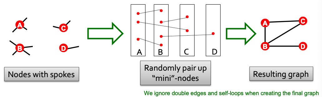
New Model: Configuration Model
- Goal: Generate a random graph with a given degree sequence
- Useful as a “null” model of networks:
- We can compare the real network and a “random” which has the same degree sequence as
- Configuration model:
Alternative for Spokes: Switching
- Start from a given graph G
- Repeat the switching step times:
- Select a pair of edges at random
- Exchange the endpoints to give
- Exchange edges only if no multiple edges or self-edges are generated
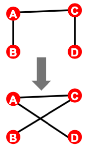
- Result: A randomly rewired graph:
- Same node degrees, randomly rewired edges
- Q is chosen large enough (e.g., Q=100) for the process to converge
Motif Significance Overview
- Intuition: Motifs are overrepresented in a network when compared to random graphs:
- Step 1: Count motifs in the given graph
- Step 2: Generate random graphs with similar statistics (e.g. number of nodes, edges, degree sequence), and count motifs in the random graphs
- Step 3: Use statistical measures to evaluate how significant is each motif
- Use Z-score
Z-score for Statistical Significance
- captures statistical significance of motif :
- is # (motif ) in graph
- is average # (motif ) in random graph instances
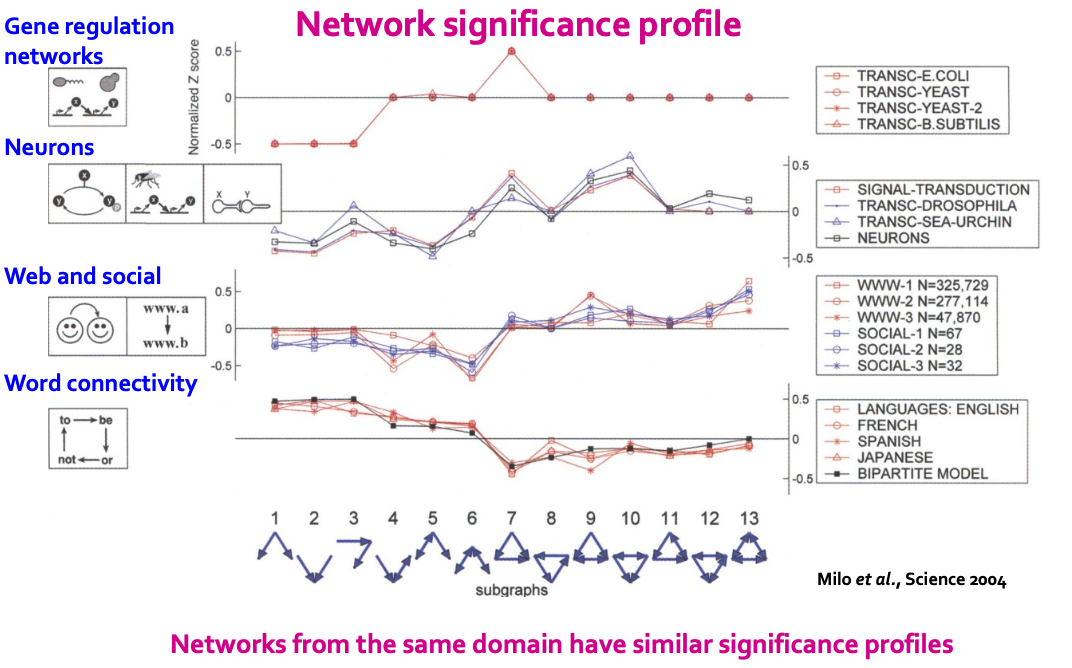
- Network significance profile (SP):
- SP is a vector of normalized Z-scores
- The dimension depends on number of motifs considered
- SP emphasizes relative significance of subgraphs:
- Important for comparison of network of different sizes
- Generally, larger graphs display higher Z-scores.
Significance Profile
- For each subgraph:
- Z-score metric is capable of classifying the subgraph “significance”:
- Negative values indicate under-representation
- Positive values indicate over-representation
- Z-score metric is capable of classifying the subgraph “significance”:
- We create a network significance profile:
- A feature vector with values for all subgraph types
- Example SP
Neural Subgraph Representations
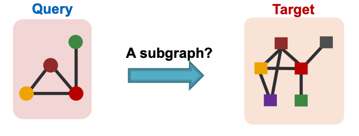
Subgraph Matching
- Given:
- Large target graph (can be disconnected)
- Query graph (connected)
- Decide:
- Is a query graph a subgraph in the target graph?
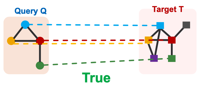
Node colors indicate the correct mapping of the nodes.
- Use GNN to predict subgraph isomorphism.
- Intuition: Exploit the geometric shape of embedding space to capture the properties of subgraph isomorphism
- Task Setup
- Consider a binary prediction: Return True if query is isomorphic to a subgraph of the target graph, else return False.
- Task Setup
Overview of the Approach
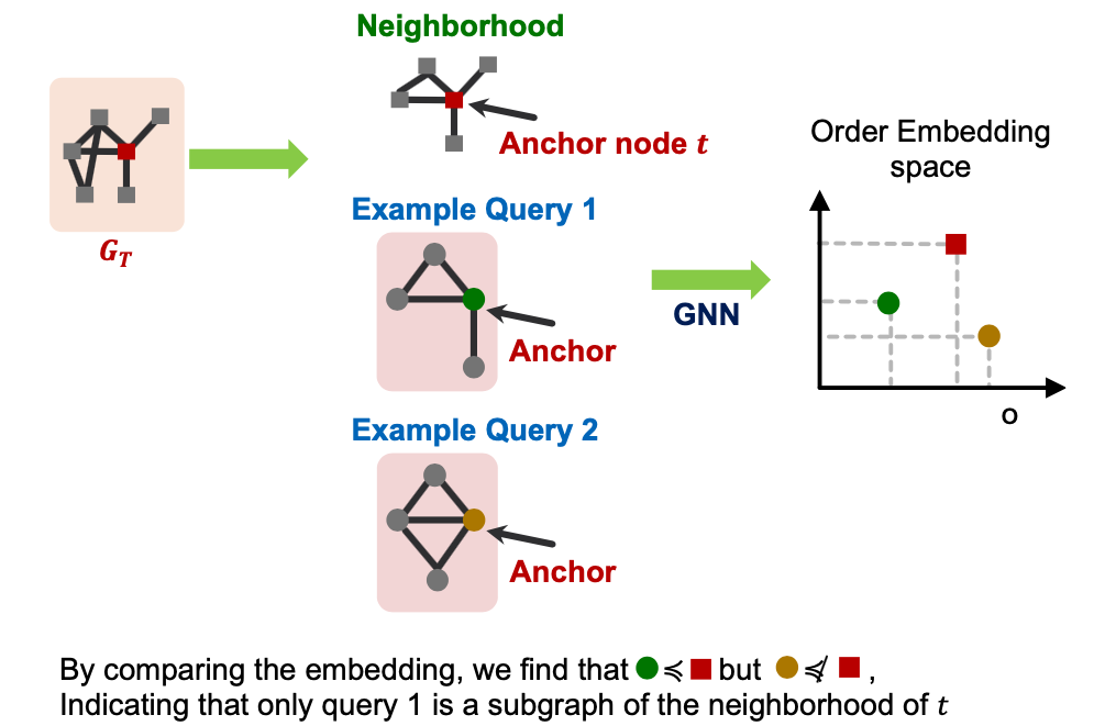
We are going to work with node-anchored definitions:
We are going to work with node-anchored neighborhoods:
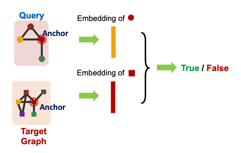
Use GNN to obtain representations of and
Predict if node ’s neighborhood is isomorphic to node neighborhood:
Why Anchor?
- Recall node-level frequency definition: The number of nodes in for which some subgraph of is isomorphic to and the isomorphism maps to .
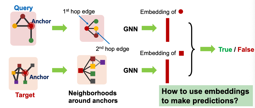
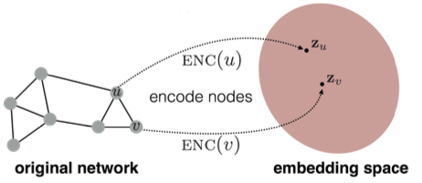
- We can compute embeddings for and using GNN
- Use embeddings to decide if neighborhood of is isomorphic to subgraph of neighborhood of
- We not only predict if there exists a mapping, but also a identify corresponding nodes ( and )!
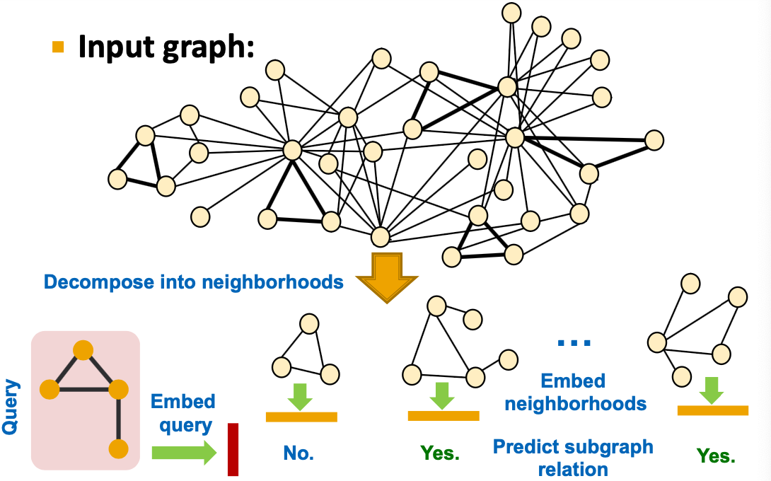
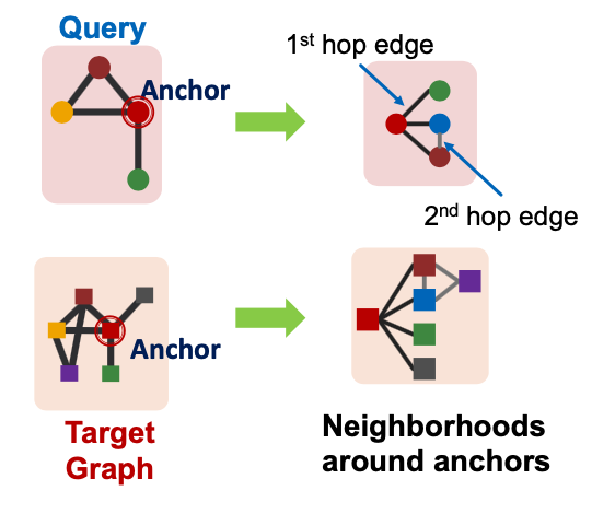
Decomposing into Neighborhoods
- For each node in :
- Obtain a k-hop neighborhood around the anchor
- Can be performed using breadth-first search (BFS)
- The depth is a hyper-parameter (e.g. 3)
- Larger depth results in more expensive model
- Same procedure applies to to obtain the neighborhoods
- We embed the neighborhoods using a GNN
- By computing the embeddings for the anchor nodes in therir respective neighborhoods.
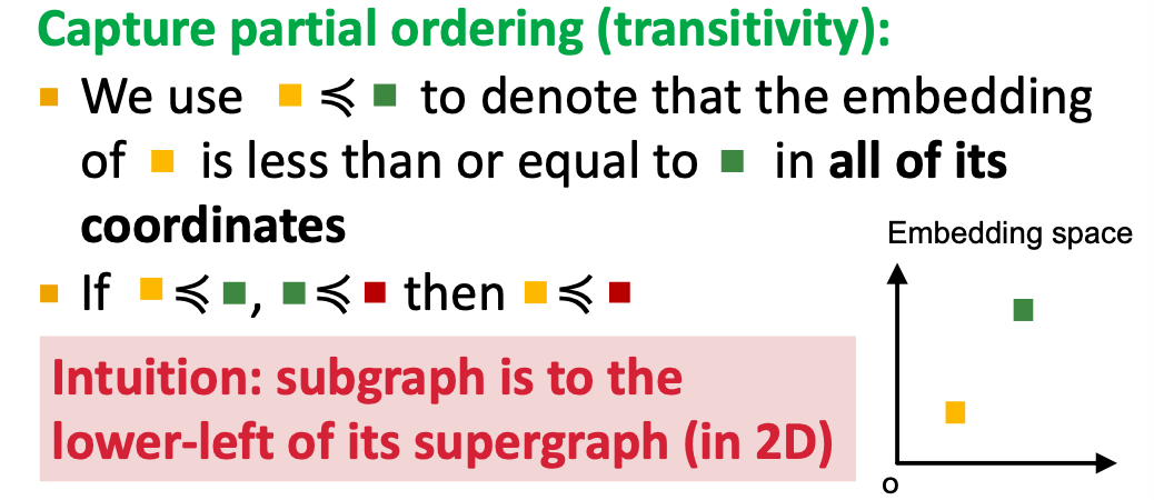
Idea: Order Embedding Space
Map graph to a point into a high-dimensional (e.g. 64-dim) embedding space, such that is non-negative in all dimensions.
Subgraph Order Embedding Space
Why Order Embedding Space?
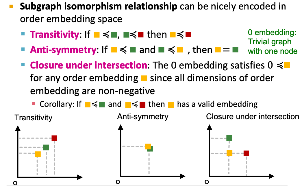
Subgraph isomorphism relationship can be nicely encoded in order embedding space
- Transitivity: If is a subgraph of , is a subgraph of , then is a subgraph of
- Anti-symmetry: If is a subgraph of , and is a subgraph of , then is isomorphic to .
- Closure under intersection: The trivial graph of 1 node is a subgraph of any graph.
- All properties have their counter-parts in the order embedding space.
- Example:
Order Constraint
- We use a GNN to learn to embed neighborhoods and preserve the order embedding structure.
- What loss function should we use, so that the learned order embedding reflects the subgraph relationship?
- We design loss functions based on the order constraint:
- Order constraint specifies the idea order embedding property that reflects subgraph relationships.
- We specify the order constraint to ensure that the subgraph properties are preserved in the order embedding space.
Order Constraint: Loss Function
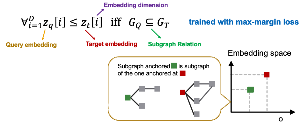
- GNN Embeddings are learned by minimizing a max-margin loss
- Define as the “margin” between graphs and
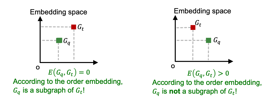
- To learn the correct order embeddings, we want to learn such that
- when is a subgraph of .
- when is not a subgraph of .
Training Neural Subgraph Matching
- To learn such embeddings, construct training examples where half the time, is a subgraph of , and the other half, it is not.
- Train on these examples by minimizing the following max-marging loss:
- For positive examples: Minimize when is a subgraph of
- For negative example: Minnimize
- Max-margin loss prevents the model from learning the degenerate strategy of moving embeddings further and further apart forever.
Training Example Construction
- Need to generate training queries and targets from the dataset
- Get by choosing a random anchor and taking all nodes in within distance from to be in .
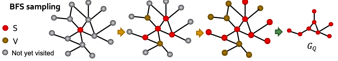
- Postive examples: Sample induced subgraph of . Use BFS sampling:
- Initialize
- Let be all neihbors of nodes in . At every step, sample of the nodes in , put them in . Put the remaining nodes of in .
- After steps, take the subgraph of induced by anchored at
- Negative examples( not subgraph of ): “corrupt” by adding/removing nodes/edges so it’s no longer a subgraph.
Details:
- How many training examples to sample?
- At every iteration, we sample new training pairs
- Benefit: Every iteration, the model sees different subgraph examples
- Improves performance and avoids overfitting - since there are exponential number of possible subgraphs to sample from.
- How deep is the BFS sampling?
- A hyper-parameter that trades off runtime and performance.
- Usually use 3-5, depending on size of the dataset.
Subgraph Predictions on New Graphs
- Given: query graph anchored at node , target graph anchored at node .
- Goal: Output whether the query is a node-anchored subgraph of the target.
- Procedure:
- If , predict “True”; else “False”
- is a hyper-parameter.
- To check if is isomorphic to a subgraph of , repeat this procedure for all . Here is the neighborhood around node .
Finding Frequent Subgraphs
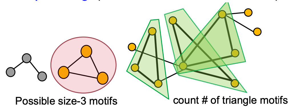
Generally, finding the most frequent size- motifs requires solving two challenges:
- Enumerating all size connected subgraphs
- Counting # (occurrences of each subgraph type)
- Subgraph isomorphism is NP-complete
- Feasible motif size for traditional methods is relatively small (3 to 7)
Finding frequent subgraph patterns is computationally hard
- Combinatorial explosion of number of possible patterns
- Counting subgraph frequency is NP-hard
Representation learning can tackle these challenges:
- Combinatorial explosion → Organize the search space
- Subgraph isomorphism → Prediction using GNN
Representation learning can tackle these challenges:
- Counting # (occurrences of each subgraph type)
- Solution: Use GNN to “predict” the frequency of the subgraph.
- Enumerating all size- connected subgraphs
- Solution: Don’t enumerate subgraphs but construct a size- subgraph incrementally
- Note: We are only interested in high frequency subgraphs
- Solution: Don’t enumerate subgraphs but construct a size- subgraph incrementally
Problem Setup: Frequent Motif Mining
- Target graph (dataset) , size parameter
- Desired number of results
- Goal:: Identify, among all possible graphs of nodes, the graphs with the highest frequency in .
- We use the node-level definition: The number of nodes in for which some subgraph of is isomorphic to and the isomorphism maps to .
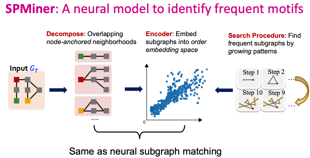
SPMiner: Key Idea
- Decompose input graph into neighborhoods
- Embed neighhborhoods into an order embedding space
- Key benefit of order embedding: We can quickly “predict” the frequency of a given subgraph
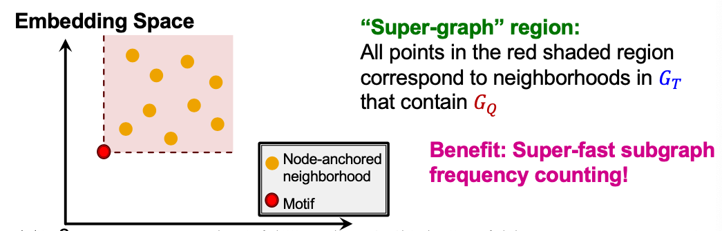
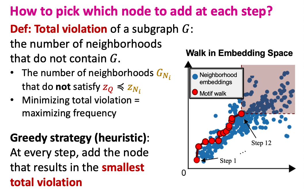
Motif Frequency Estimation
- Given: Set of subgraphs (”node-anchored neighborhoods”) of (sampled randomly)
- Key idea: Estimate frequency of by counting the number of such taht their embeddings satisfy
- This is a consequence of the order embedding space property
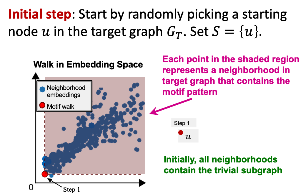
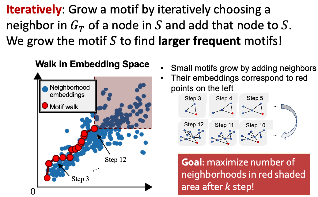
SPMiner Search Procedure
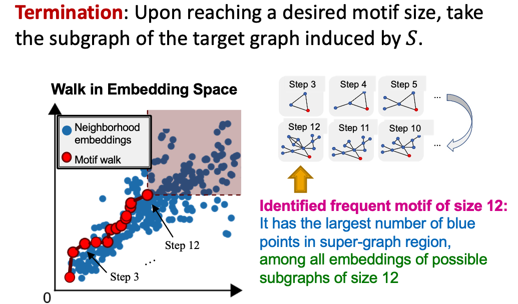
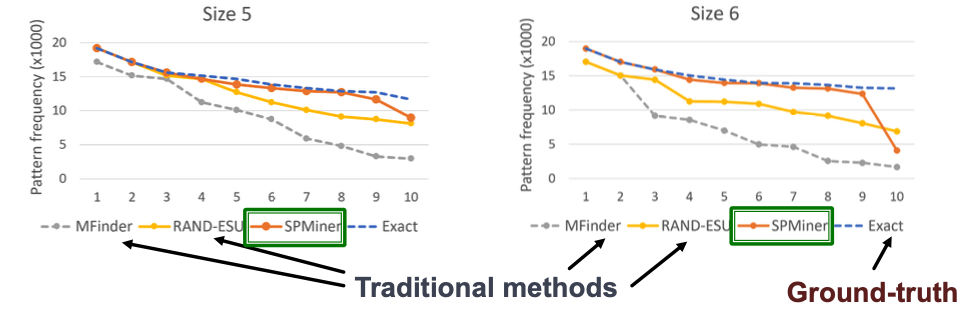
Results: Small Motifs
- Ground-truth: Find most frequent 10 motifs in dataset by brute-force exact enumeration (expensive)
- Question: Can the model identify frequent motifs?
- Result: The model identifies 9 and 8 of the top 10 motifs, respectively.