CS224W-Machine Learning with Graph-GNNs for Recommender Systems
Recommender Systems: Task and Evaluation
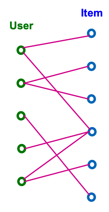
Recommender system can be naturally modeled as a bipartite graph
- A graph with two node types users and items.
- Edges connect users and items
- Indicates user-item interaction
- Often associated with timestamp
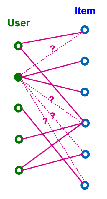
Recommendation Task
- Given: Past user-item interactions
- Task
- Predict new items each user will interact in the future
- Can be cast as link prediction problem.
- Predict new user-item interaction edges given the past edges.
- For , we need to get a real-valued score
Modern Recommender System
- Problem: Can not evaluate for every user - item pair.
- Solution: 2-stage process:
- Candidate generation (cheap, fast)
- Ranking (slow, accurate)
Top- Recommendation
For each user, we recommend items.
- For recommendation to be effective, needs to be much smaller than the total number of items (up to billions)
- is typically in the order of 10-100.
The goal is to include as many positive items as possible in the top- recommended items.
- Positive items = Items that the user will interact with in the future.
Evaluation metric: Recall @ (defined next)
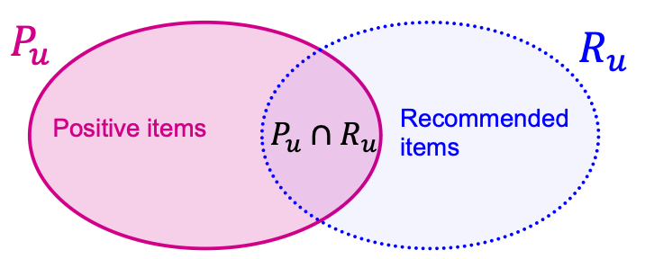
- For each use ,
- Let be a set of positive items the user will interact in the future.
- Let be a set of items recommended by the model.
- In top- recommendation, .
- Items that the user has already interacted are excluded.
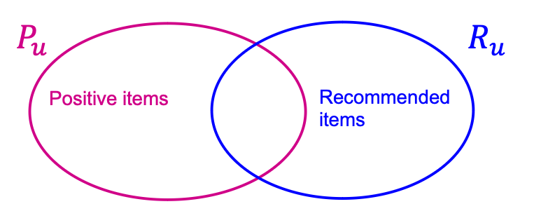
- Recall @ for user is
- Higher value indicates more positive items are recommended in top- for user .
- The final Recall @ is computed by averaging the recall values across all users.
Recommender Systems: Embedding - Based Models
Notation:
- : A set of all users
- : A set of all items
- : A set of observed user-item interactions
-
Score Function
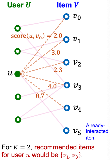
To get the top- items, we need a score function for user-item interaction:
- For , we need to get a real-valued scalar .
- items with the largest scores for a given user (excluding already-interacted items) are then recommended.
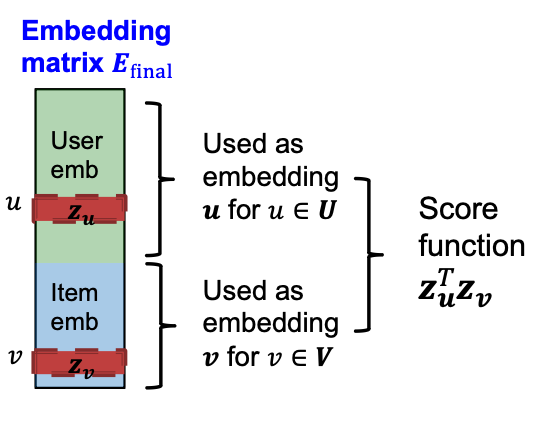
Embedding - Based Models
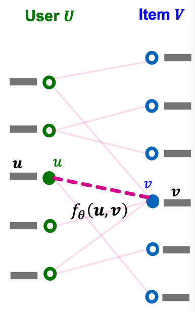
We consider embedding-based models for scoring user-item interactions.
- For each user , let be its -dimensional embedding.
- For each item , let be its -dimensional embedding.
- Let be a parameterized function.
- Then,
Training Objective
Embedding-based models have three kinds of parameters:
- An encoder to generate user embeddings
- An encoder to generate item embeddings
- Score function
Training objective: Optimize the model parameters to achieve high recall @ on seen (i.e., training) user-item interactions
- We hope this objective would lead to high recall @ on unseen (i.e., test) interactions
Surrogate Loss Functions
The original training objective (recall @ ) is not differentiable.
- Can not apply efficient gradient-based optimization
Two surrogate loss functions are widely-used to enable efficient gradient-based.
- Binary loss
- Bayesian Personalized Ranking (BPR) loss
Surrogate losses are differentiable and should align will with the original training objective.
Binary Loss
- Define positive/negative edges
- A set of positive edges (i.e., observed/training user-item interactions)
- A set of negative edges
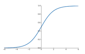
- Define sigmoid function
- Maps real-valued scores into binary linkelihood scores, i.e., in the range of
- Binary loss: Binary classification of positive / negative edges using
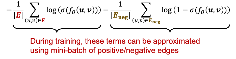
- Binary loss pushes the scores of positive edges higher than those of negative edges.
- This aligns with the training recall metric since positive edges need to be recalled.
- Issue: In the binary loss, the scores of ALL positive edges are pushed higher than those of ALL negative edges.
- This would unnecessarily penalize model predictions even if the training recall metric is perfect.
- Why?
- Consider the simplest case:
- Two users, two items
- Metric: Recall @ 1.
- A model assigns the score for every user-item pair (as shown in the right)
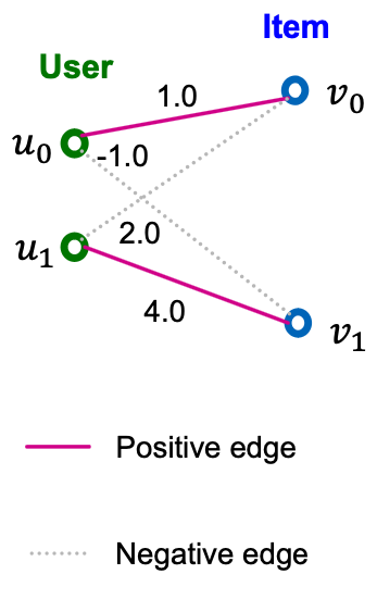
- Training Recall @1 is 1.0, because (resp. ) is correctly recommended to . (resp. ).
- However, the binary loss would still penalize the model prediction because the negative edge gets the higher score than the positive edge .
- Consider the simplest case:
- Key insight: The binary loss is non-personalized in the sense that the positive /negative edges are considered across ALL users at once.
- However, the recall metric is inherently personalized (defined for each user)
- The non-personalized binary loss is overly-stringent for the personalized recall metric.
Desirable Surrogate Loss
- Surrogate loss function should be defined in a personalized manner.
- For each user, we want the scores of positive items to be higher than those of the negative items.
- We do not care about the score ordering across users.
- Bayesian Personalized Ranking (BPR) loss achieves this!
Loss Function: BPR Loss
- Bayesian Personalized Ranking (BPR) loss is a personalized surrogate loss that aligns better with the recall @ metric.
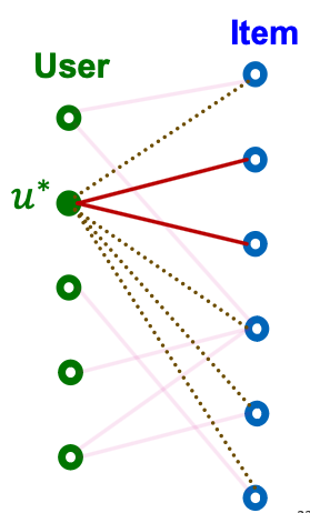
- For each user , define the rooted positive / negative edges as
- Positive edges rooted at
-
- Negative edge rooted at
-
- Positive edges rooted at
- Training objective: For each user , we want the scores of rooted positive edges to be higher than those of rooted negative edges
- Aligns with the personalized nature of the recall metric.
- BPR Loss for user :
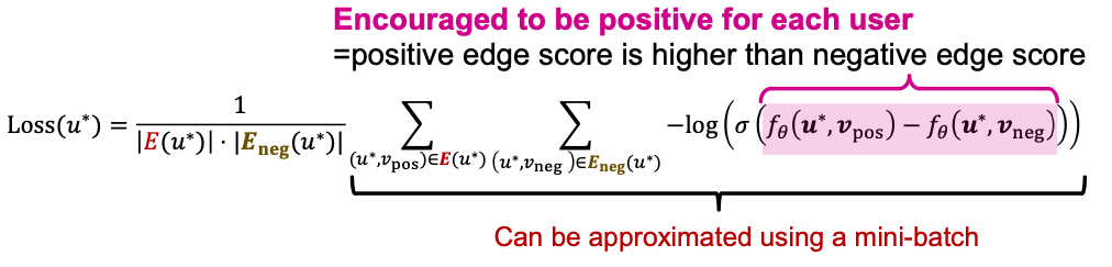
- Final BPR Loss:
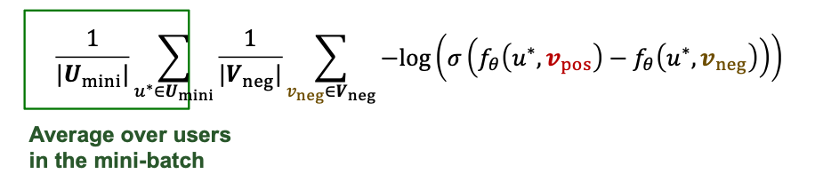
- Mini-batch training for the BPR loss:
- In each mini-batch, we sample a subset of users
- For each user we sample one postive item and a set of sampled negative itmes .
- The mini-batch loss is computed as
- In each mini-batch, we sample a subset of users
Why Embedding Models Work?
- Underlying idea: Collaborative filtering
- Recommend items for a user by collecting preferences of many other similar users.
- Similar users tend to prefer similar items.
- Key question: How to capture similarity between users / items?
- Embedding-based models can capture similarity of users/items!
- Low-dimensional embeddings cannot simply memorize all user-item interaction data.
- Embeddings are forced to capture similarity between users/items to fit the data.
- This allows the models to make effective prediction on unseen user-item interactions.
Neural Graph Collaborative Filtering
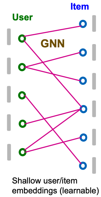
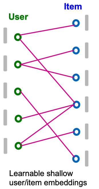
Conventional Collaborative Filtering
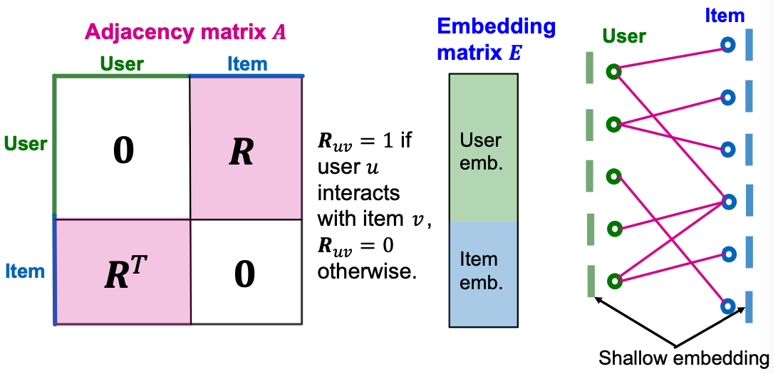
- Conventional collaborative filtering model is based on shallow encoders:
- No user/item features.
- Use shallow encoders for users and items:
- For every and , we prepare shallow learnable embeddings .
- Score function for user and item is .
Limitations of Shallow Encoders
- The model itself does not explicitly capture graph structure.
- The graph structure is only implicitly captured in the training objective.
- Only the first-order graph structure (i.e., edges) is captured in the training objective.
- High-order graph structure (e.g., -hop paths between two nodes) is not explicitly captured.
NGCF: Overview
- Neural Graph Collaborative Filtering (NGCF) explicitly incorporates high-order graph structure when generating user /item embeddings.
- Key idea: Use a GNN to generate graph-aware user/item embeddings.
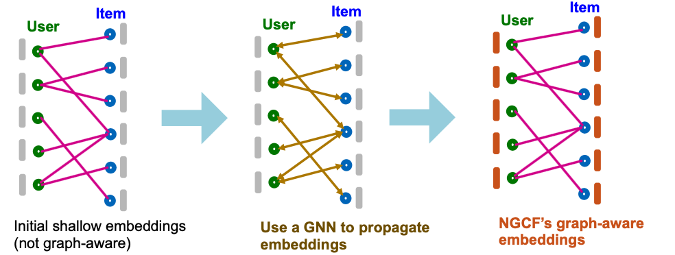
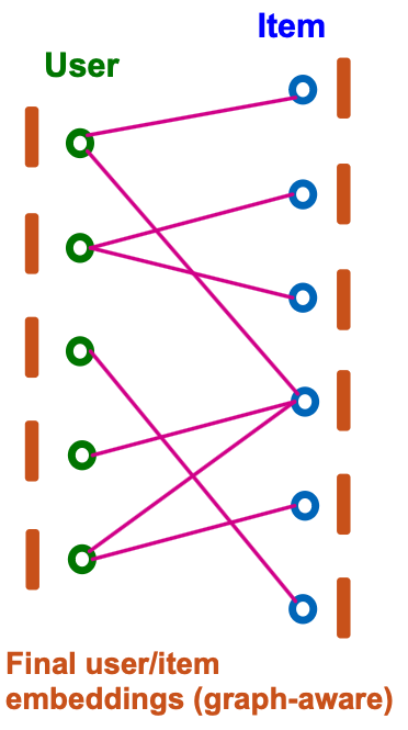
NGCF Framework
- Given: User-item bipartite graph.
- NGCF framework:
- Prepare shallow learnable embedding for each node.
- Use multi-layer GNNs to propagate embeddings along the bipartite graph.
- High-order graph structure is captured.
- Final embeddings are explicitly graph-aware!
- Two kinds of learnable params are jointly learned:
- Shallow user/item embeddings
- GNN’s parameters
Initial Node Embeddings
- Set the shallow learnable embeddings as the initial node features:
- For every user , set as the user’s shallow embedding.
- For every item , set as the item’s shallow embedding.
Neighbor Aggregation
- Iteratively update node embeddings using neighboring embeddings.
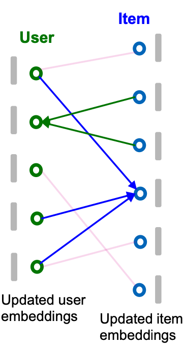
High-order graph structure is captured through iterative neighbor aggregation.
Different architecture choices are possiblle for AGGR and COMBINE
- can be
- can be
Final Embeddings and Score Function
- After rounds of neighbor aggregation, we get the final user/item embeddings and .
- For all , we set
- Score function is the inner product
- Recall: NGCF jointly learns two kinds of parameters:
- Shallow user /item embeddings
- GNN’s parameters
- Observation: Shallow learnable embeddings are already quite expressive.
- learned for every node
- Most of the parameter counts are in shallow embeddings
- The GNN parameters may not be so essential for performance.
- Overview of the idea:
- Adjacency matrix for a bipartite graph
- Matrix formulation of GCN
- Simplification of GCN by removing non-linearity
- Related: SGC for scalable GNN.
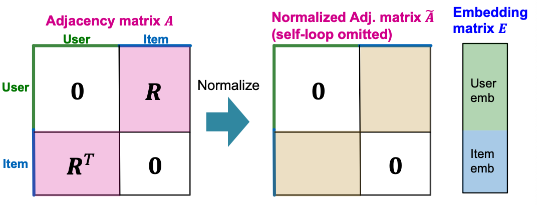
Adjacency and Embedding Matrices
- Adjacency matrix of a (undirected) bipartite graph.
- Shallow embedding matrix.
Matrix Formulation of GCN
- Define: The diffusion matrix
- Let be the degree matrix of .
- Define the norrmalized adjacency matrix as
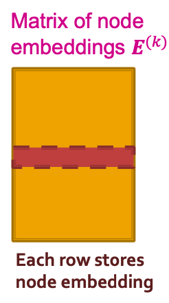
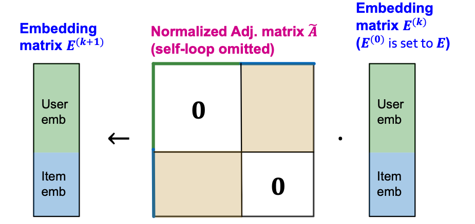
- Let be the embedding matrix at -th layer.
- Each layer of GCN’s aggregation can be written in a matrix form:
- : Neighbor aggregation
- : Learnable linear transformation
Note: Different from the original GCN, self-connection is omitted here.
Simplifying GCN
- Simplify GCN by removing ReLU non-linearity:
- The final node embedding matrix is given as:
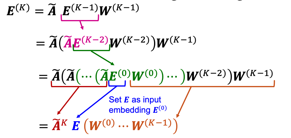
- Removing ReLU significantly simplifies GCN!
- : Diffusing node embeddings along the graph
- Algorithm: Apply for times.
- Each matrix multiplication diffuses the current embeddings to their non-hop neighbors.
- Note: is dense and never gets materialized. Instead, the above iterative matrix-vector product is used to compute
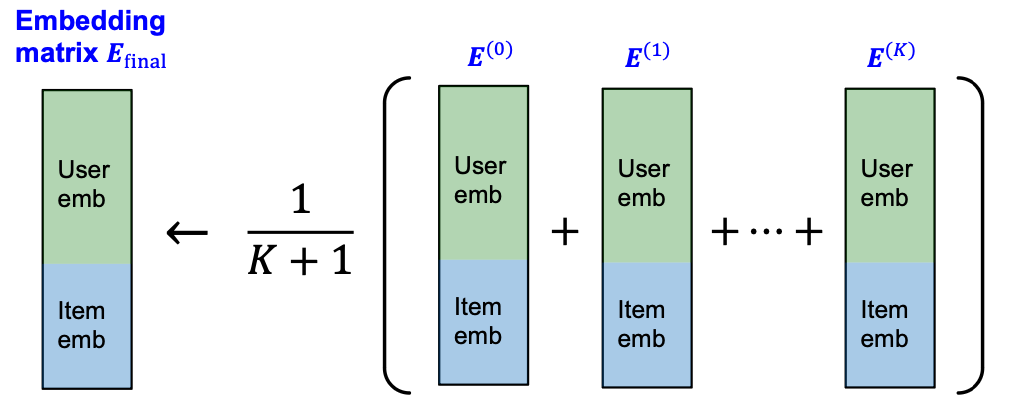
Multi-Scale Diffusion
- We can consider multi-scale diffusion
- The above includes embeddings diffused at multiple hop scales.
- acts as a self-connection (that is omitted in the definition )
- The coefficients, , are hyper-parameters.
- For simplicity, LightGCN uses the uniform coefficient, i.e., for .
LightGCN: Model Overview
Given:
- Adjacency matrix
- Initial learnable embedding matrix
Iteratively diffuse embedding matrix using . For
Average the embedding matrices at different scales.
Score function:
- Use user/item vectors from to score user-item interaction
LightGCN: Intuition
- Question: Why does the simple diffusion propagation work well?
- Answer: The diffusion directly encourages the embeddings of similar users / items to be similar.
- Similar users share many common neighbors(items) and are expected to have similar future preferences (interact with similar items).
LightGCN and GCN
- The embedding propagation of LightGCN is closely related to GCN
- Recall: GCN (neighbor aggregation part)
- Self-loop is added in the neighborhood definition
- LightGCN uses the same equation except that
- Self-loop is not added in the neighborhood definition.
- Final embedding takes the average of embeddings from all the layers:
LightGCN and MF: Comparison
- Both LightGCN and shallow encoders learn a unique embedding for each user/item.
- The difference is that LightGCN uses the diffused user/item embeddings for scoring.
- LightGCN performs better than shallow encoders but are also more computationally expensive due to the additional diffusion step.
- The final embedding of a user/item is obtained by aggregating embeddings of its multi-hop neighboring nodes.
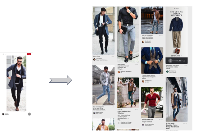
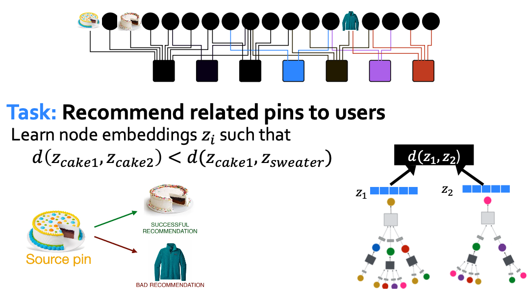
Motivation
P2P recommendation
PinSAGE: Pin Embedding
- Unifies visual, textual, and graph information.
- The largest industry deployment of a Graph Convolutional Networks.
- Huge Adoption across Pinterest
- Works for fresh content and is available in a few seconds after pin creation.
Application: Pinterest
PinSage graph convolutional network:
- Goal: Generate embeddings for nodes in a large-scale Pinterest graph containing billions of object.
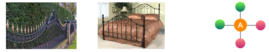
- Key Idea: Borrow information from nearby nodes.
- E.g., bed rail Pin might look like a garden fence, but gates and beds are rarely adjacent in the graph.
- Pin embeddings are essential to various tasks like recommendation of Pins, classification, ranking
- Services like “Related Pins”, ”Search”, ”Shopping”, “Ads”
Harnessing Pins and Boards
PinSAGE: Graph Neural Network
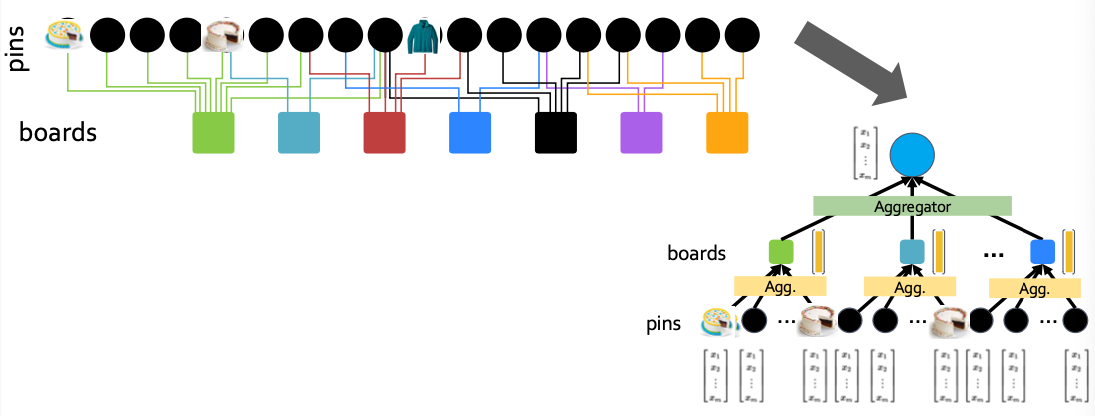
- Graph has tens of billions of nodes and edges
- Further resolves embeddings across the Pinterest graph
PinSAGE: Methods for Scaling Up
In addition to the GNN model, the PinSAGE introduces several methods to scale the GNN to a billion-scale recommender system (e.g., Pinterest).
- Shared negative samples across users in a mini-batch
- Hard negative samples
- Curriculum learning
- Mini-batch training of GNNs on a large-graph
PinSAGE Model
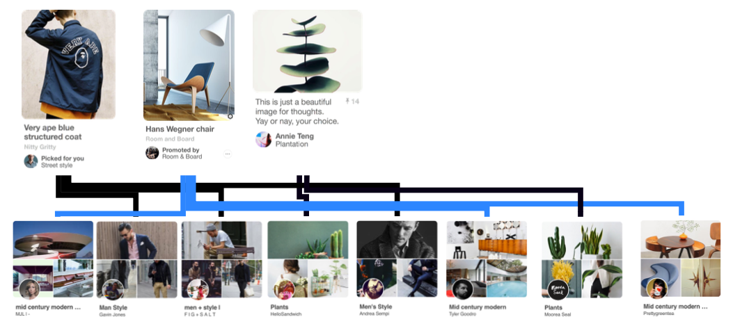
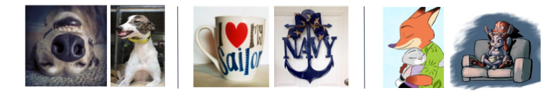
Training Data
- 1+B repin pairs:
- From Relation Pins surface
- Capture semantic relatedness
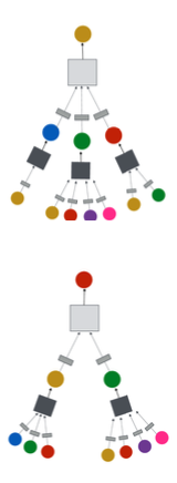
- Goal: Embed such pairs to be “neighbors”
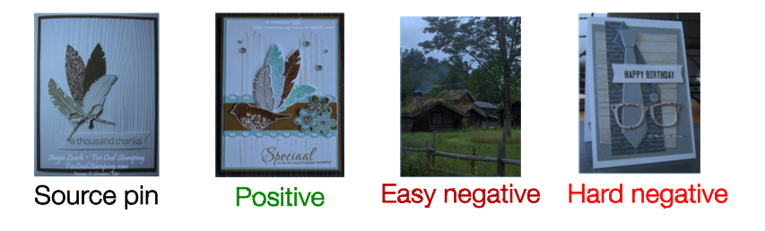
- Example positive training pairs(Q,X):
Shared Negative Samples
- Recall: In BPR loss, for each user , we sample one positive item and a set of sampled negative items
- Using more negative samples per user improves the recommendation performance, but it also expensive.
- We need to generate embeddings for negative nodes.
- We need to apply GNN computational graphs (see down), which is expensive.
- Key idea: We can share the same set of negative samples across all users in the mini-batch.
- This way, we only need to generate embeddings for negative nodes.
- This saves the node embedding generation computation by a factor of !
- Empirically, the performance stays similar to the non-shared negative sampling scheme.
PinSAGE: Curriculum Learning
- Idea: use harder and harder negative samples
- Include more and more hard negative samples for each epoch
- Key insight: It’s effective to make the negative samples gradually harder in the process of training.
- At -th epoch, we add hard negative items.
- # (Hard negatives) gradually increases in the process of training.
- The model will gradually learn to make finer-grained predictions.
- At -th epoch, we add hard negative items.
Hard Negatives 1
- Challenge: Industrial recsys needs to make extremely fine-grained predictions.
- #Total items: Up to billions
- #Items to recommend for each user:: 10 to 100.
- Issue: The shared negative items are randomly sampled from all items
- Most of them are “easy negatives”, i.e., a model does not need to be fine-grained to distinguish them from positive items.
- We need a way too sample “hard negatives” to force the model to be fine-grained! (看上面的Curriculum Learning)
Hard Negatives 2
- For each user node, the hard negatives are item nodes that are close (but not connected) to the user node in the graph.
- Hard negatives for user are obtained as follows:
- Compute random walks from user .
- Run random walk with restart from , obtain visit counts for other items/nodes.
- Sort items in the descending order of their visit count.
- Randomly sample items that are ranked high but not too high, e.g., .
- Item nodes that are close but not too close (connected) to the user node.
- Compute random walks from user .
- The hard negatives for each user are used in addition to the shared negatives.
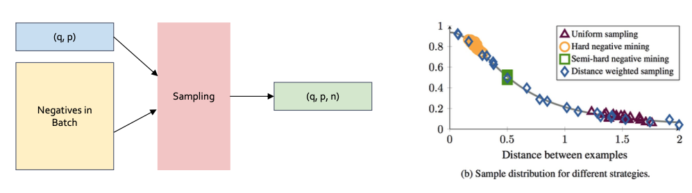
PinSAGE: Negative Sampling
positive pairs are given but various methods to sample negative to form
- Distance Weighted Sampling
- Sample negatives so that query-negative distance distribution is approx