CS224W-Machine Learning with Graph-Advanced Topics in Graph Neural Network
Limitations of Graph Neural Networks
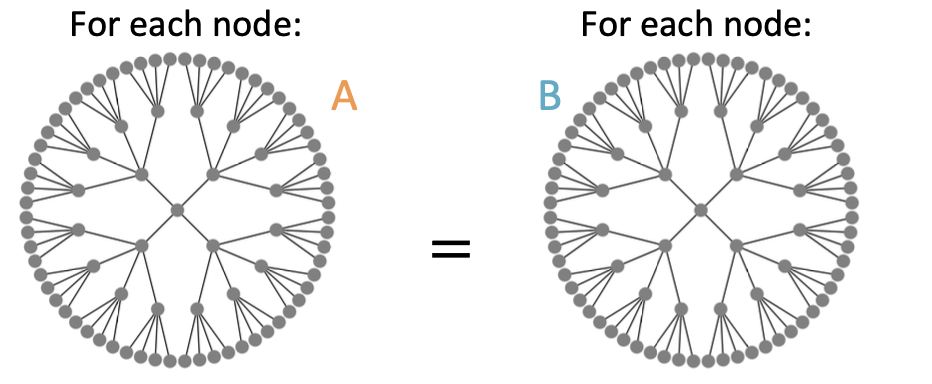
A “Perfect” GNN Model (一些缺点)
- A thought experiment: What should a perfect GNN do?
- A -layer GNN embeds a node based on the -hop neighborhood structure
- A perfect GNN should build an injective function between neighborhood structure (regrdless of hops) and node embeddings.
- Therefore, for a perfect GNN:
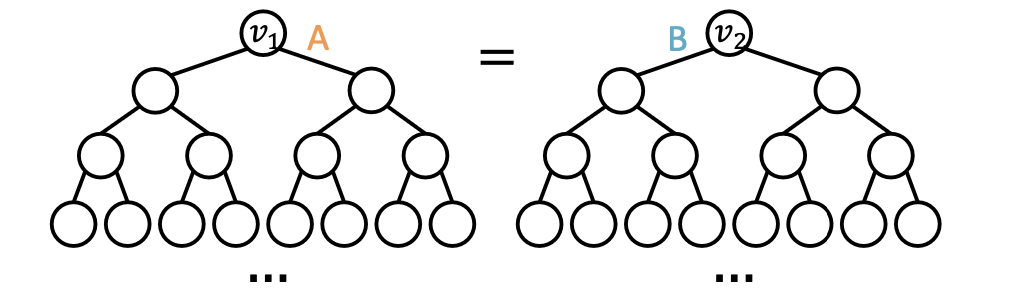
- Observation 1: If two nodes have the same neighborhood structure, they must have the same embedding
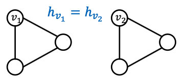
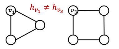
- Observation 2: If two nodes have different neighborhood structure, they must have different embeddings
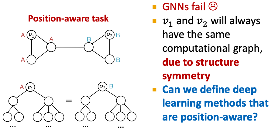
Imperfections of Existing GNNs
- However, Observations 1 & 2 are imperfect.
- Observation 1 could have issues:
- Even though two nodes may have the same neighborhood structure, we may want to assign different embeddings to them.
- Because these nodes appear in different positions in the graph
- We call these tasks Position-aware tasks.
- Even a perfect GNN will fail for these tasks:
- Observation 2 often can not be satisfied:
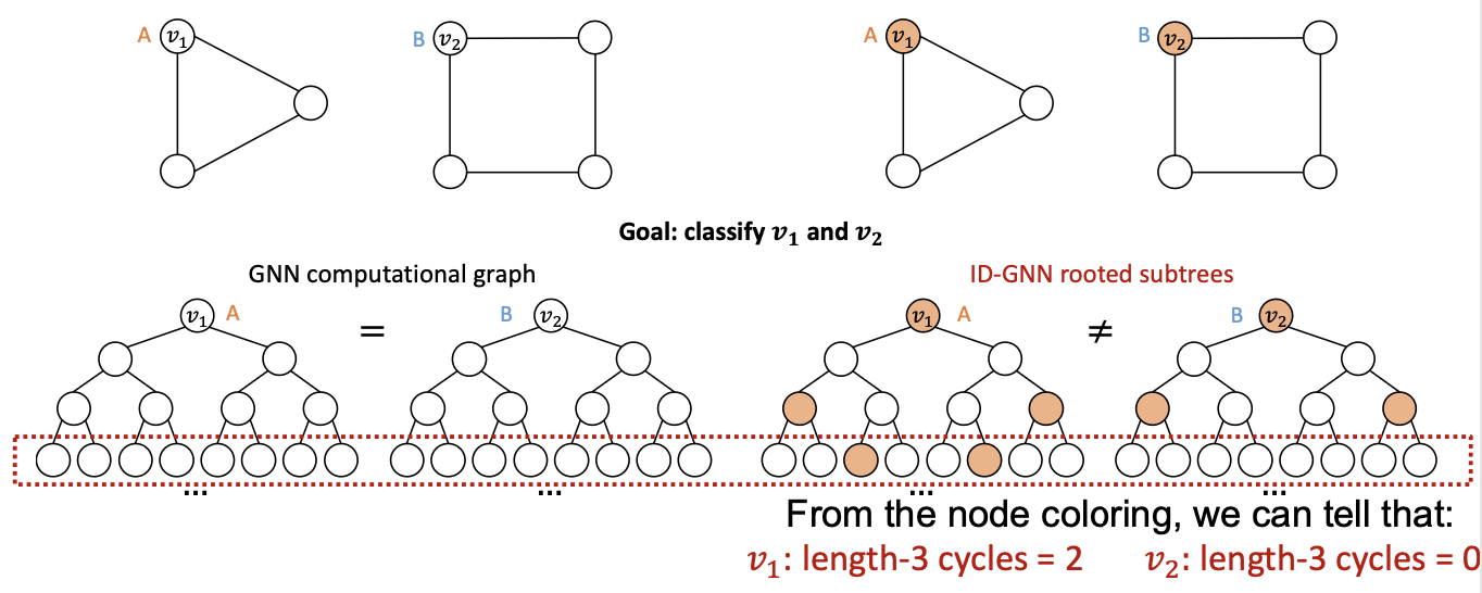
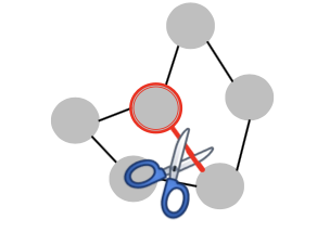
- The GNNs we have introduced so far are not perfect
- In Lecture 9(Reasoning), we discussed that their expressive power is upper bounded by the WL test
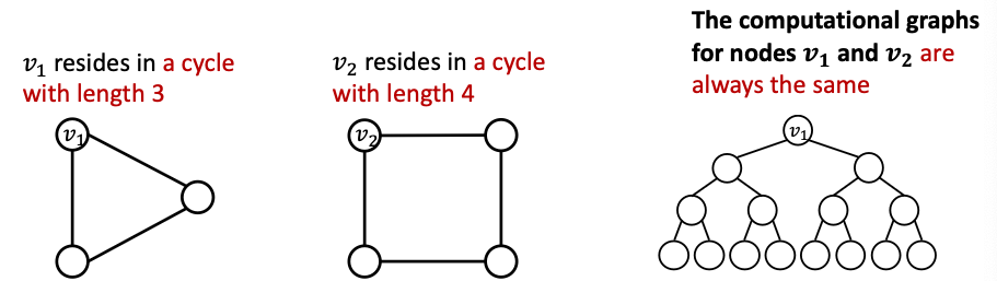
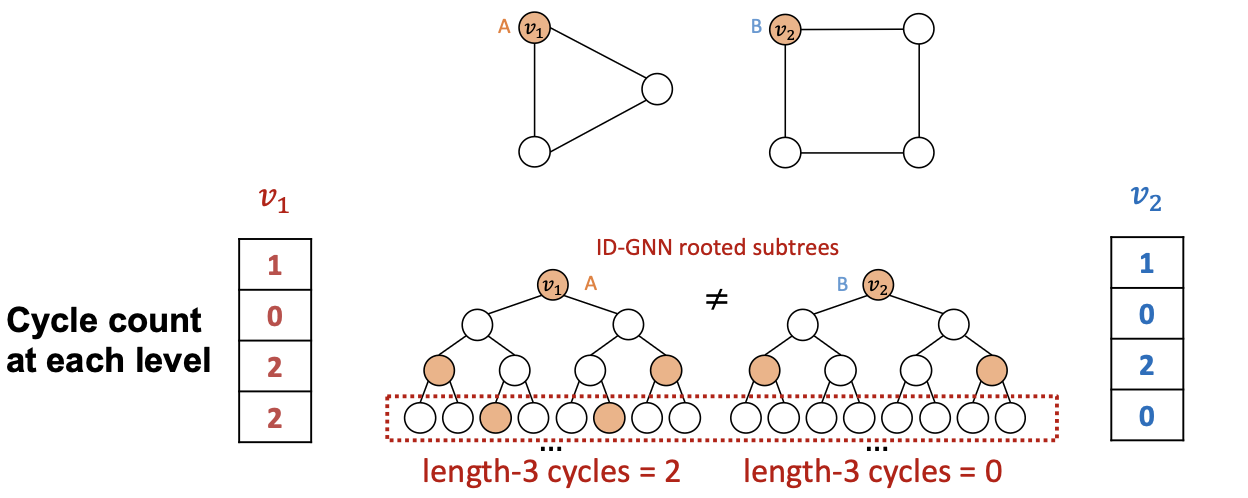
- For example, message passing GNNs cannot count the cycle length:
- Fix issues in Observation 1:
- Create node embeddings based on their positions in the graph.
- Example method: Position-arware GNNs
- Fix issues in Observation 2:
- Build message passing GNNs that are more expressive than WL test.
- Example method: Identity-aware GNNs
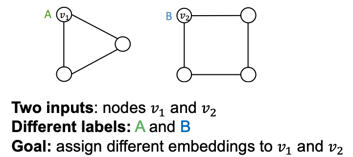
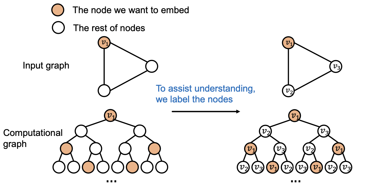
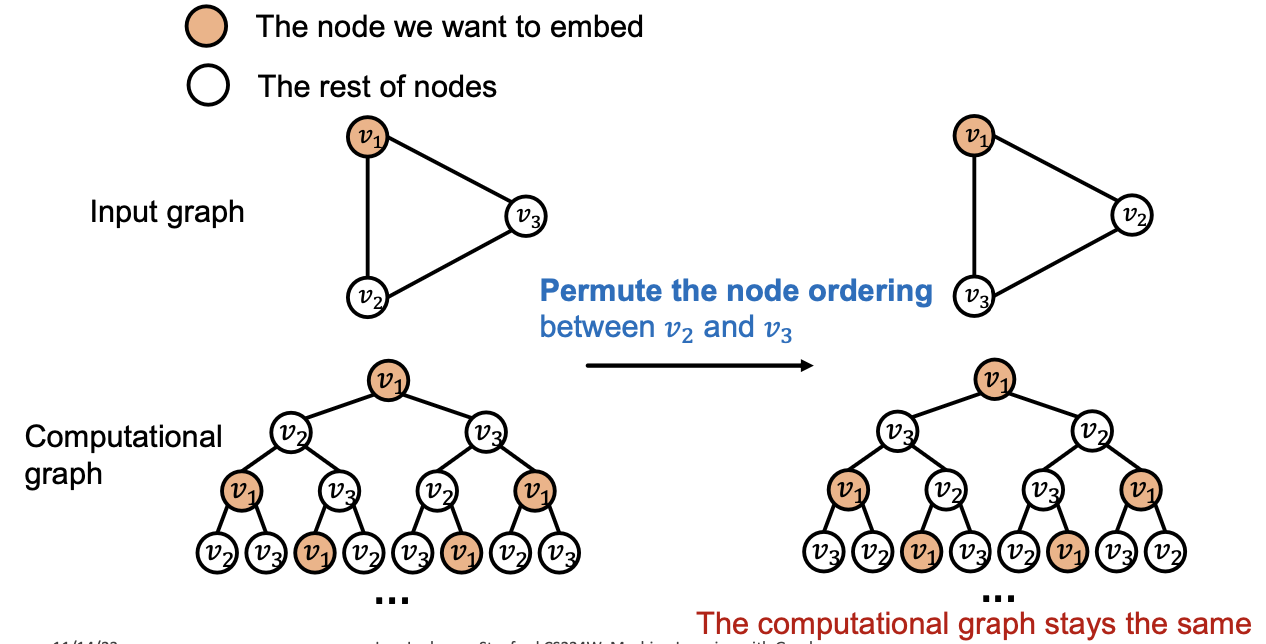
Our Approach
- We use the following thinking:
- Two different inputs (nodes, edges, graphs) are labeled differently
- A “failed” model will always assign the same embedding to them
- A “successful” model will assign different embeddings to them
- Embeddings are determined by GNN computational graphs:
Naive Solution is not Desirable
- A naive solution: One-hot encoding
- Encode each node with a different ID, then we can always differentiate different nodes/ edges / graphs
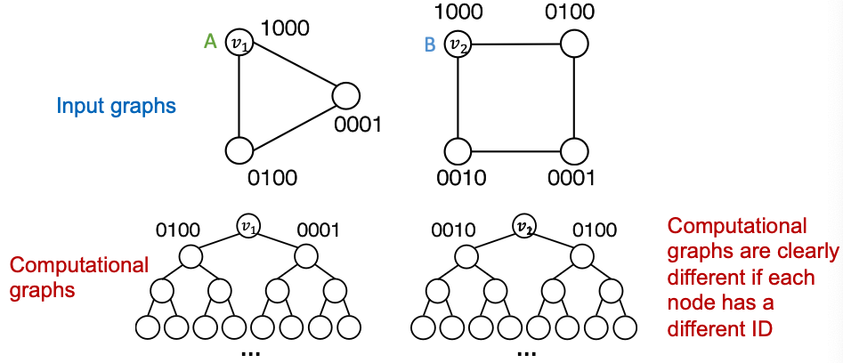
- Issues:
- Not scalable: Need feature dimensions ( is the number of nodes)
- Not inductive: Cannot generalize to new nodes/graphs
Position-aware Graph Neural Networks
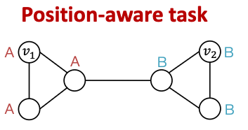
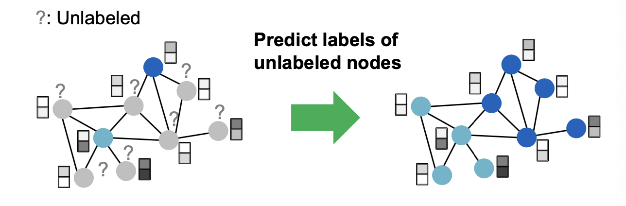
Two Types of Tasks on Graphs (Postion-aware GraphNN)
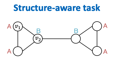
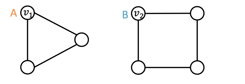
- Nodes are labeled by their structural roles in the graph.
- GNNs often work well for structure-aware tasks
- Nodes are labeled by their positions in the graph.
- GNNs will always fail for position-aware tasks
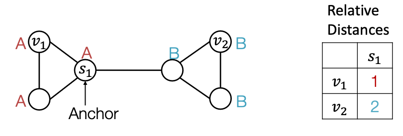
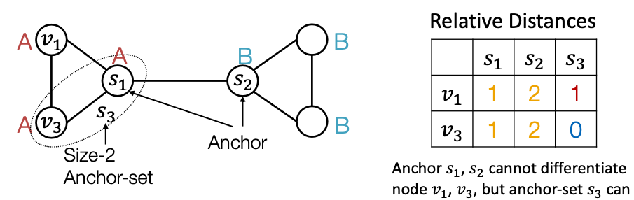
Power of “Anchor”
- Randomly pick a node as an anchor node
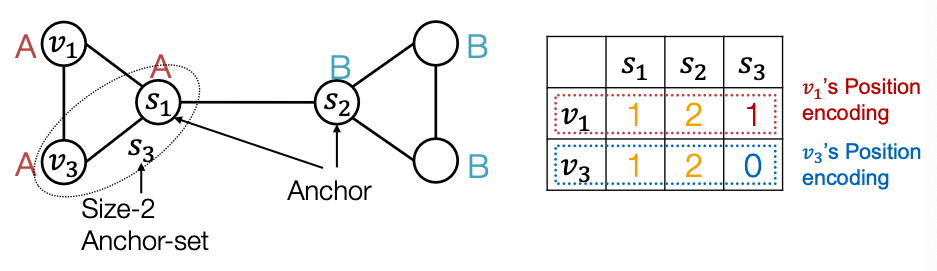
- Represent and via their relative distances w.r.t. the anchor , which are different.
- An anchor node serves as a coordinate axis
- Which can be used to locate nodes in the graph
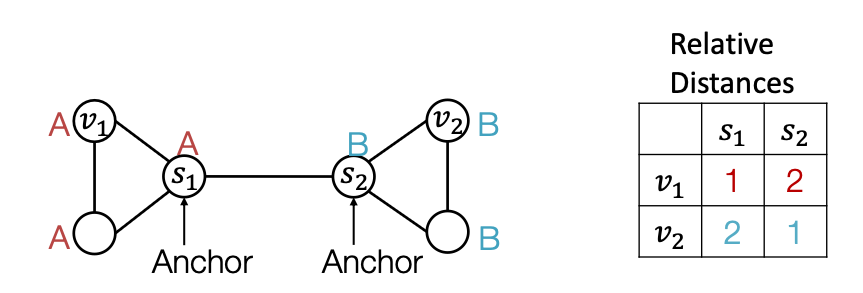
- Pick more ndoes as anchor nodes
- Observation: More anchors can better characterize node position in different regions of the graph
- Many anchors Many coordinate axes
Power of “Anchor-sets”
- Generalize anchor from a single node to a set of nodes
- We define distance to an anchor-set as the minimum distance to all the nodes in the ancho-set.
- Observation: Large anchor-sets can sometimes provide more precise position estimate
- We can save the total number of anchors.
Anchor Set: Theory
- Goal: Embed the metric space into the Euclidian space such that the original distance metric is preserved.
- For every node pairs , the Euclidian embedding distance is close to the original distance metric .
- Bourgain Theorem [Informal]
- Consider the following embedding function of node .
- where
- is a constant.
- is chosen by including each node in independently with probability
-
- The embedding distance produced by is provably close to the original distance metric .
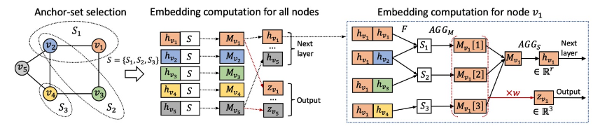
- P-GNN follows the theory of Bourgain theorem
- First samples anchor sets .
- Embed each node via
- P-GNN maintains the inductive capability
- During training, new anchor sets are re-sampled every time.
- P-GNN is learned to operate over the new anchor sets.
- At test time, given a new unseen graph, new anchor sets are sampled.
- Position encoding for graphs: Represent a node’s position by its distance to randomly selected anchor-sets
- Each dimension of the position encoding is tied to an anchor set
How to use position information?
- This simple way: Use position encoding as an augmented node feature (works well in practice)
- Issue: Since each dimension of position encoding is tied to a random anchor set, dimensions of positional encoding can be randomly permuted, without changing its meaning
- Imagine you permute the input dimensions of a normal NN, the output will surely change.
- The rigorous solution: Requires a special NN that can maintain the permutation invariant property of position encoding
- Permuting the input feature dimension will only result in the permutation of the output dimension, the value in each dimension won’’t change
- Position-aware GNN paper has more details.
Identity-Aware Graph Neural Networks
- GNNs would fail for position-aware tasks.
- GNN can not perform perfectly in structure-aware tasks
- GNNs exhibit three levels of failure cases in structure-aware tasks:
- Node level
- Edge level
- Graph level
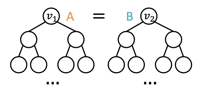
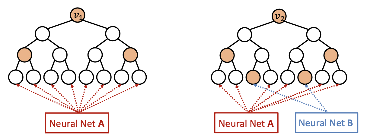
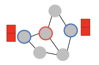
Different Inputs but the same computational graph → GNN fails
GNN Failure 1: Node-level Tasks
Example input graphs
Existing GNNs’ computational graphs
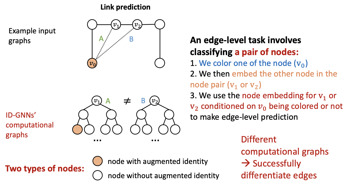
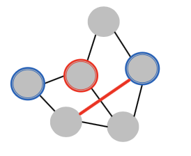
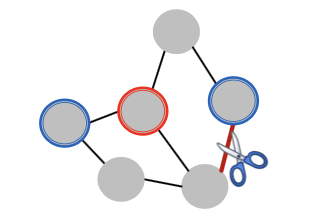
GNN Failure 2: Edge-level Tasks
Example input graphs
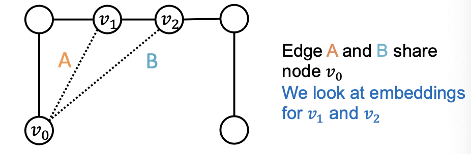
Existing GNNs’ computational graphs
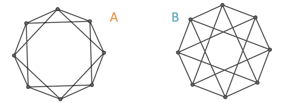
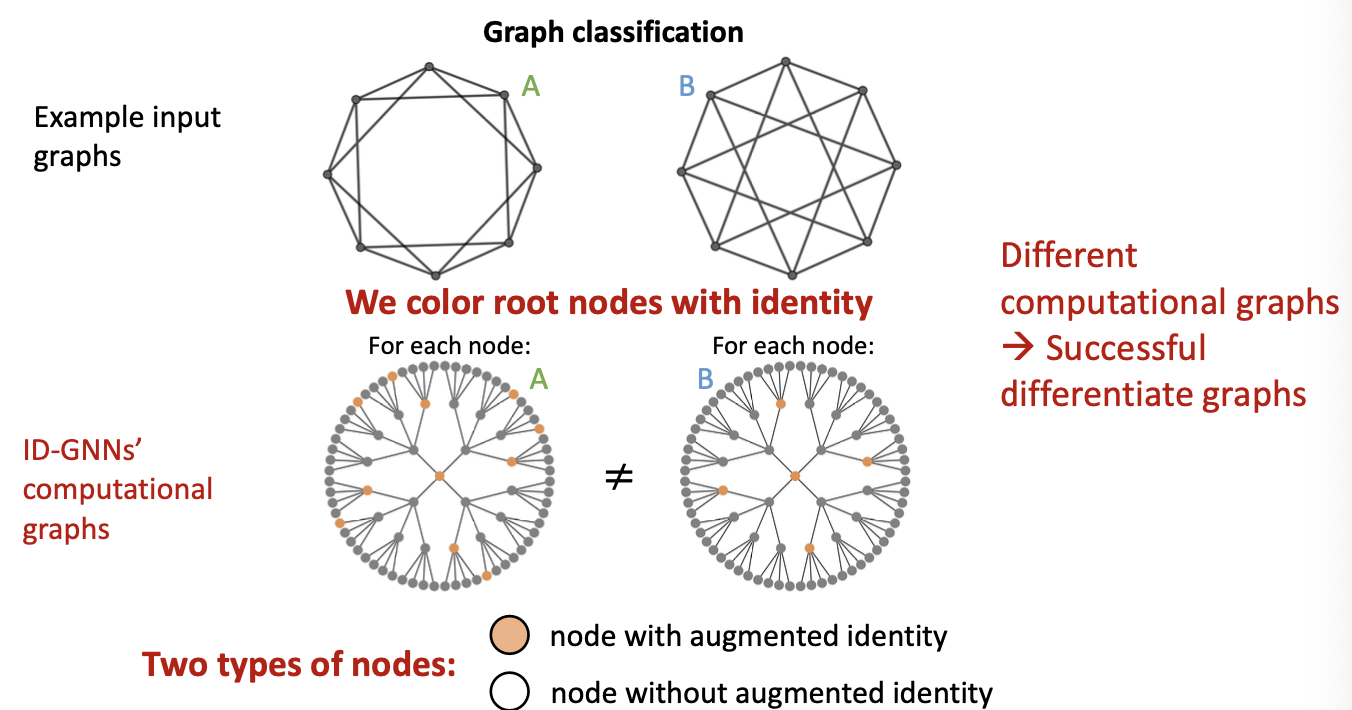
GNN Failure 3: Graph-level Tasks
Example input graphs
We look at embeddings for each node
Existing GNNs’ computational graphs
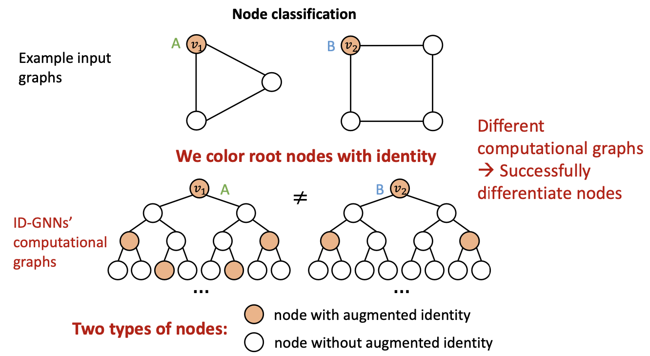
Idea: Inductive Node Coloring
Idea: We can assign a color to the node we want to embed
- This coloring is inductive:
- It is invariant to node ordering / identities
Inductive Node Coloring - Node Level
- Inductive node coloring can help node classification
Inductive Node Coloring - Edge Level
- Inductive node coloring can help link prediction
Inductive Node Coloring - Graph Level
- Inductive node coloring can help graph classification
How to build a GNN using node coloring?
- Utilize inductive node coloring in embedding computation
- Idea: Heterogenous message passing
- Normally, a GNN applies the same message / aggregation computation to all the nodes.
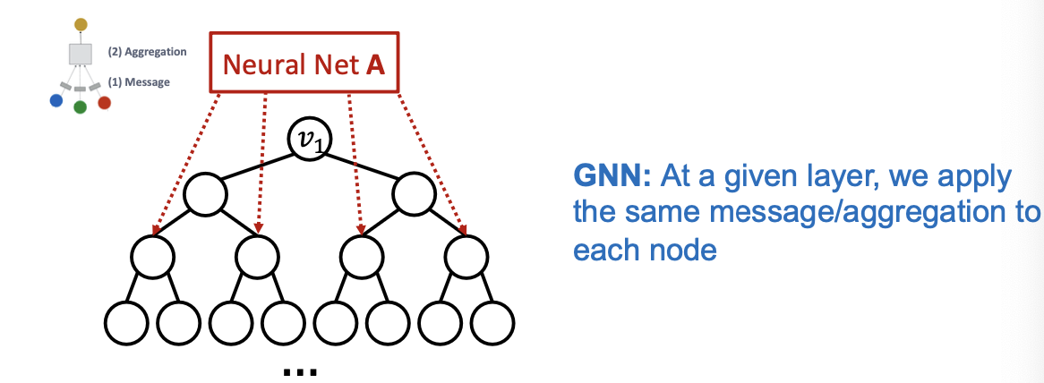
- Heterogenous: Different types of message passing is applied to different nodes.
- An ID-GNN applies different message / aggregation to nodes with different colorings.
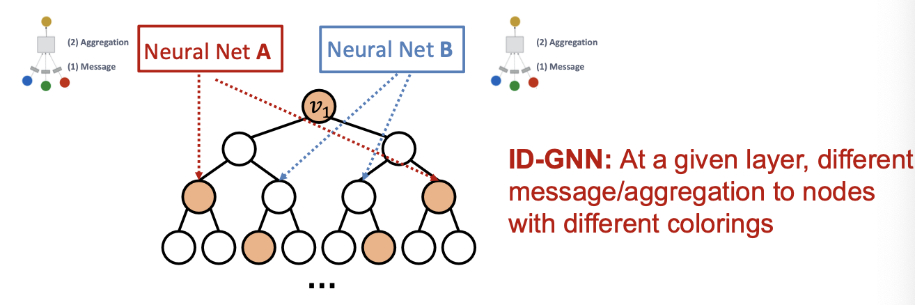
- Idea: Heterogenous message passing
Identity-aware GNN
- Output: Node embedding for .
- Step 1: Extract the ego-network
- : - hop neighborhood graph around
- Set the initial node feature
- For , (input node feature)
- Step 2: Heterogeneous message passing
- For do
- For do
Depending on whether ( in the center node ) or not , we use different neural network functions to transform .
- For do
- Why does heterogenous message passing work:
- Suppose two node have the same computational graph structure, but have different node colorings
- Since we will apply different neural network for embedding computation, their embeddings will be different
- GNN vs. ID-GNN
- Why does ID-GNN work better than GNN?
- Intuition: ID-GNN can count cycles originating from a given node, but GNN cannot.
- Why does ID-GNN work better than GNN?
- Simplified Version: ID-GNN-Fast
- Based on the intuition, we present a simplified version ID-GNN-Fast.
- Include identity information as an augmented node feature (no need to do heterogenous message passing)
- Use cycle counts in each layer as an augmented node featured. Also can be used together with any GNN
- Based on the intuition, we present a simplified version ID-GNN-Fast.
ID-GNN
- A general and powerful extension to GNN framework
- We can apply ID-GNN on any message passing GNNs (GCN, GraphSAGE, GIN, …)
- ID-GNN provides consistent performance gain in node/edge/graph level tasks.
- ID-GNN is more expressive than their GNN counterparts. ID-GNN is the first message passing GNN that is more expressive than 1-WL test
- We can easily implement ID-GNN using popular GNN tools (PyG, DGL, …)
- We can apply ID-GNN on any message passing GNNs (GCN, GraphSAGE, GIN, …)
Robustness of Graph Neural Networks
Deep Learning Performance
- Recent years have seen impressive performance of deep learning models in a variety of applications.
- Example: In computer vision, deep convolutional networks have achieved human-level performance on ImageNet (image category classification)
Adversarial Examples
- Deep convolutional neural networks are vulnerable to adversarial attacks:
- Imperceptible noise changes the prediction.
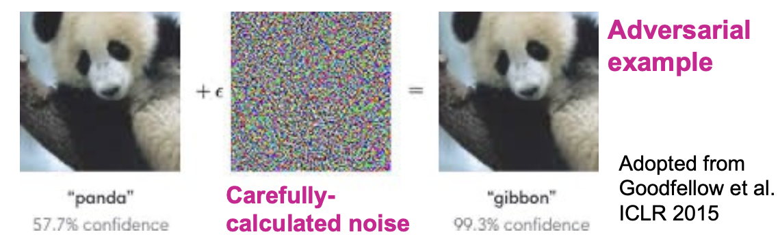
- Adversarial examples are also reported in natural language processing and audio processing domains.
Implication of Adversarial Examples
- The existence of adversarial examples prevents the reliable deployment of deep learning models to the real word.
- Adversaries may try to actively hack the deep learning models.
- The model performance can become much worse than we expect.
- Deep Learning models are often not robust.
- In fact, it is an active area of research to make these models robust against adversarial examples.
Robustness of GNNs
- How about GNNs? Are they robust to adversarial examples?
- Premise: Common applications of GNNs involve public platforms and monetary interests.
- Recommender systems
- Social networks
- Search engines
- Adversarial have the incentive to manipulate input graphs and hack GNNs’ predictions.
Setting to Study GNNs’ Robustness
- To study the robustness of GNNs, we specifically consider the following setting:
- Task: Semi-supervised node classification
- Model: GCN
Roadmap
- We first describe several real-world adversarial attack possibilities.
- We then review the GCN model that we are going to attack (knowing the opponent).
- We mathematically formalize the attack problem as an optimization problem.
- We empirically see how vulnerable GCN’s prediction is to the adversarial attack.
Attack Possibilities
- What are the attack possibilities in real world?
- Target node : node whose label prediction we want to change.
- Attacker nodes : nodes the attacker can modify
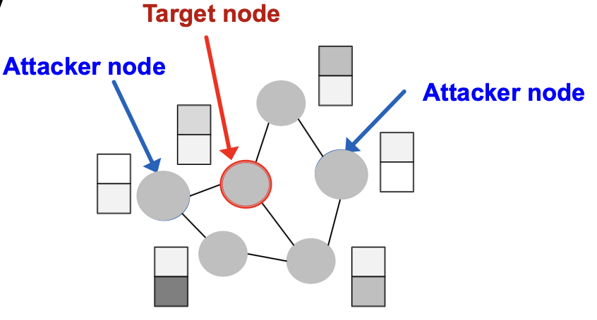
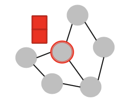
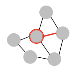
Attack Possibilities: Direct Attack
- Direct Attack: Attacker node is the target node
- Modify target node feature
- Ex) Change website content
- Add connections to target
- Ex) Buy likes/followers
- Remove connections from target
- Ex) Unfollow users
Attack Possibilities: Indirect Attack
- Indirect Attack: The target node is not in the attacker nodes:
- Modify attacker node features
- Ex) Hijack friends of targets
- Add connections to attackers
- Ex) Create a link, link farm
- Remove connections from attackers
- Ex) Delete undesirable link
Formalizing Adversarial Attacks
- Objective for the attacker:
- Maximize (change of target node label prediction)
- Subject to (graph manipulation is small)
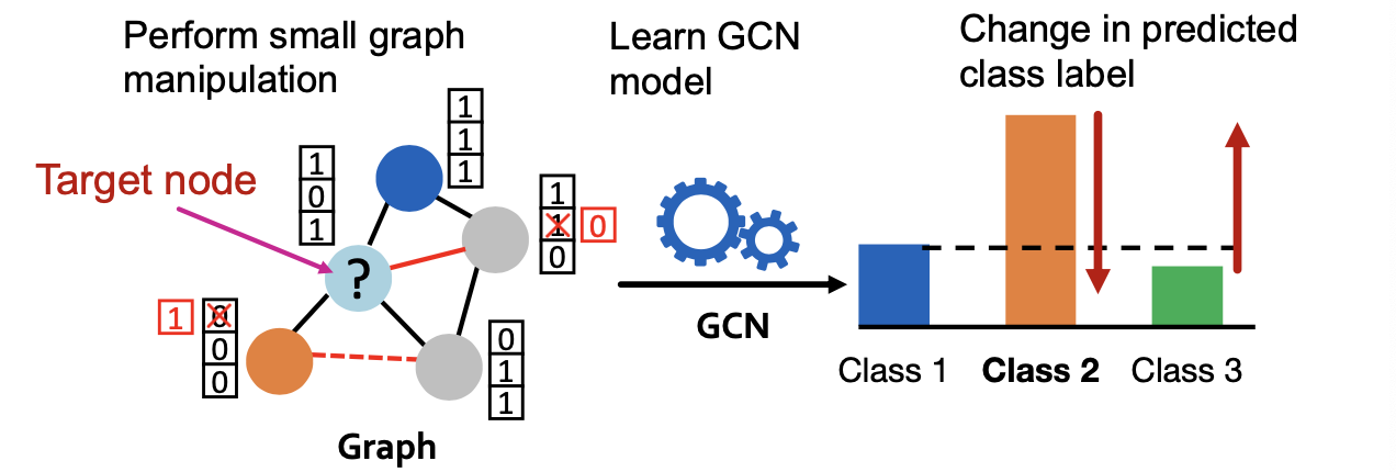
If graph manipulation is too large, it will easily be detected. Successful attacks should change the target prediction with “unnoticeably-small” graph manipulation.
Mathematical Formulation
- Original graph:
- : adjacency matrix, : feature matrix
- Manipulated graph (after adding noise):
- : adjacency matrix, : feature matrix
- Assumption:
- Graph manipulation is unnoticeably small.
- Preserving basic graph statistics (e.g, degree distribution) and feature statistics.
- Graph manipulation is either direct (changing the feature/connection of target nodes) or indirect.
- Graph manipulation is unnoticeably small.
- Overview of the attack framework
- Original adjacency matrix , node feature , node labels .
- : Model parameter learned over .
- : class label of node prediction by GCN with .
- An attacker has access to , and the learning algorithm.
- The attacker modifies into .
- : Model parameter learned over .
- : class label of node predicted by GCN with
- The goal of the attacker is to make .
- Target node:
- GCN learned over the original graph
- GCN’s original prediction on the target node:
Predict the class of vector that has the highest predicted probability.
- GCN learned over the manipulated graph
- GCN’s prediction on the target node :
- We want the prediction to change after the graph is manipulated:
- Change of prediction on target node :
- : Predicted(log) probability of the newly-predicted class . Want to increase this term
- : Predicted(log) probability of the originally-predicted class . Want to decrease this term.
- Final optimization objective:
- Challenges in optimizing the objective
- Adjacency matrix is a discrete object
- For every modified graph and , GCN needs to be retrained:
- Solution:
- Iteratively follow a locally optimal strategy:
- Sequentially ‘manipulate’ the most promising element: an entry from the adjacency matrix or a feature entry.
- Pick the one which obtains the highest difference in the log-probabilities, indicated by the score function.
- Iteratively follow a locally optimal strategy:
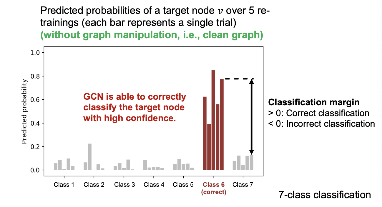
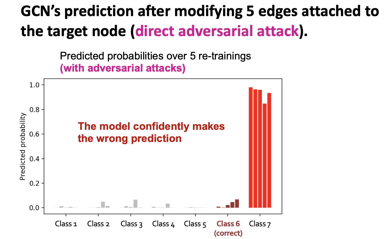
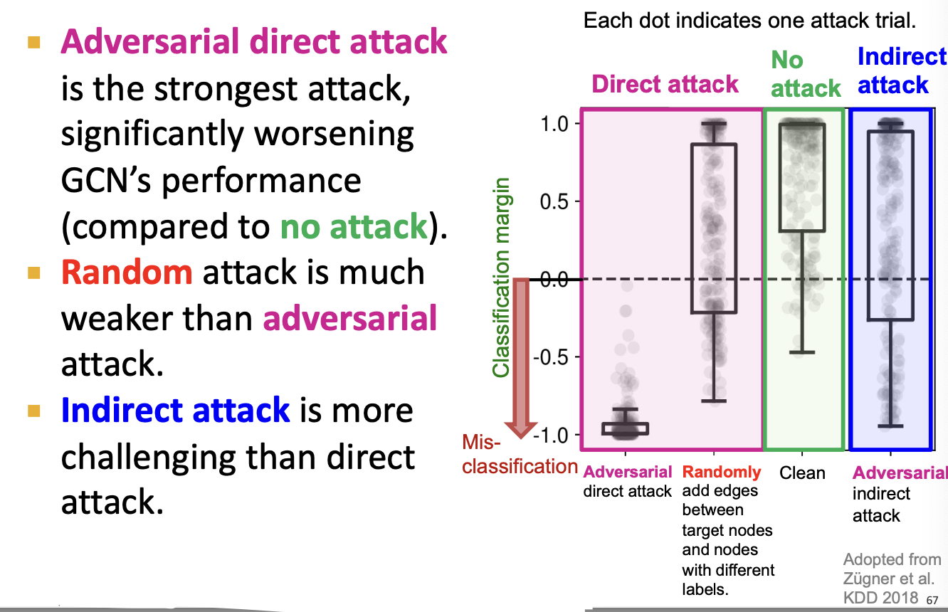
Experiments: Setting
- Setting: Semi-supervised node classification with GCN.
- Graph: Paper citation network(2800 nodes, 8000 edges).
- Attack type: Edge modification (addition or deletion of edges)
- Attack budget on node : modifications (: degree of node ).
- Intuition: It is harder to attack a node with a larger degree.
- Model is trained and attacked 5 times using different random seeds.
Experiments: Adversarial Attack