CS224W-Machine Learning with Graph-Scaling Up GNNs

• Large - Scale:
  • #nodes ranges from 10M to 10B
  • #edges ranges from 100M to 100B

• Tasks
  • Node-level: User/item/paper classification
  • Link-level: Recommendation, completion

Standard SGD cannot effectively train GNNs

• Objective: Minimize the average loss
  • $\theta$: model parameters
  • $l_i(\theta)$: loss for $i$-th data point

• We perform Stochastic Gradient Descent (SGD)
  • Sample $M(<<N)$ data points (mini-batches).
  • Compute the $l_{sub}(\theta)$ over the $M$ data points.
  • Perform SGD: $\theta \leftarrow \theta - \nabla l_{sub}(\theta)$

In mini-batch, we sample $M(<<N)$ nodes independently:

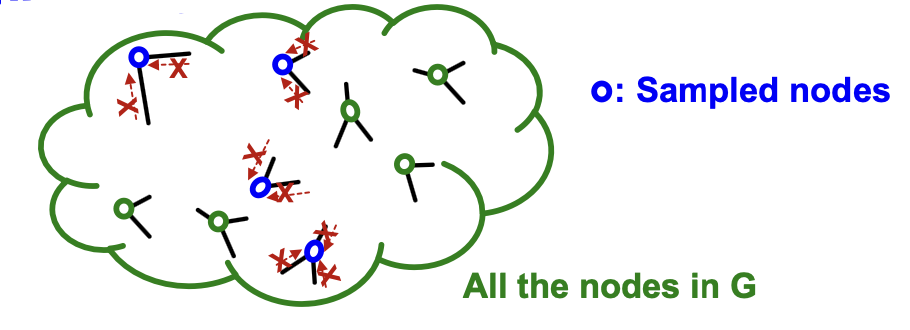
• Sampled nodes will be isolated from each other!

• GNN generates node embeddings by aggregating neighboring node features.
  • GNN does not access to neighboring nodes within the mini-batch!

Naive full-batch implementation: Generate embeddings of all the nodes at the same time:

• Load the entire graph $A$ and features $X$. Set $H^{(0)} = X$

• At each GNN layer: Compute embeddings of all nodes using all the node embeddings from the previous layer.

• Compute the loss

• Perform gradient descent

Full-batch implementation is not feasible for a large graphs. → Because we want to use GPU for fast training, but GPU memory is extremely limited (10GB - 80GB). The entire graph and the features can not be loaded on GPU.

Two methods perform message-passing over small subgraph in each mini-batch; only the subgraphs need to be loaded on a GPU at a time.

• Neighbor Sampling [Hamilton et al. NeurIPS 2017]

• Cluster-GCN [Chiang et al. KDD 2019]

One method simplifies a GNN into feature-preprocessing operation (can be efficiently performed even on a CPU)

• Simplified GCN [Wu et al. ICML 2019]
  
  
  

Sampling: Scaling up GNNs

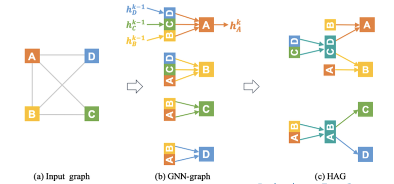
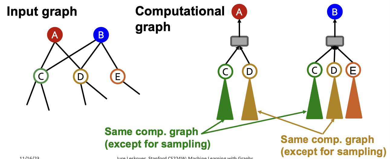
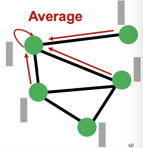
Recall: Computational Graph

• GNNs generate node embeddings via neighbor aggregation
  • Represented as a computational graph (right)

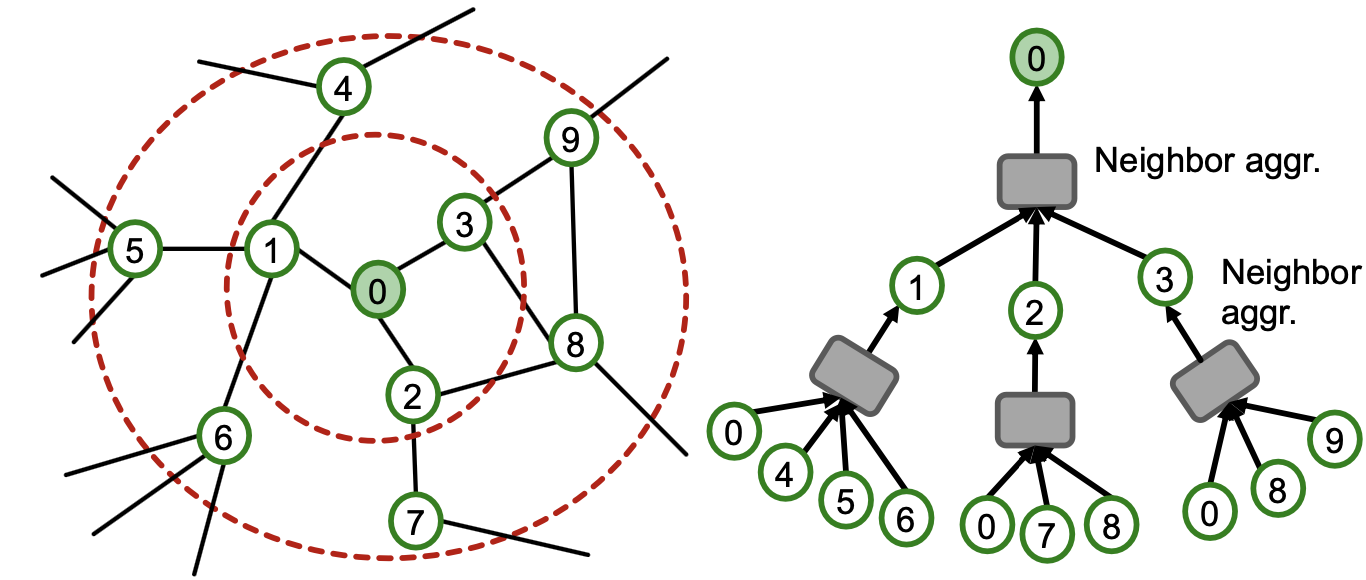
• Observation: A 2-layer GNN generates embedding of node “0” using 2-hop neighborhood structure and features

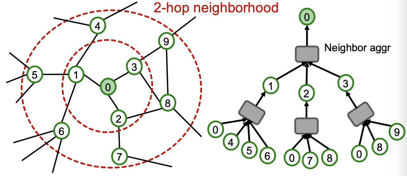
• Observation: More generally, K-layer GNNs generate embedding of a node using $K$-hop neighborhood structure and features.

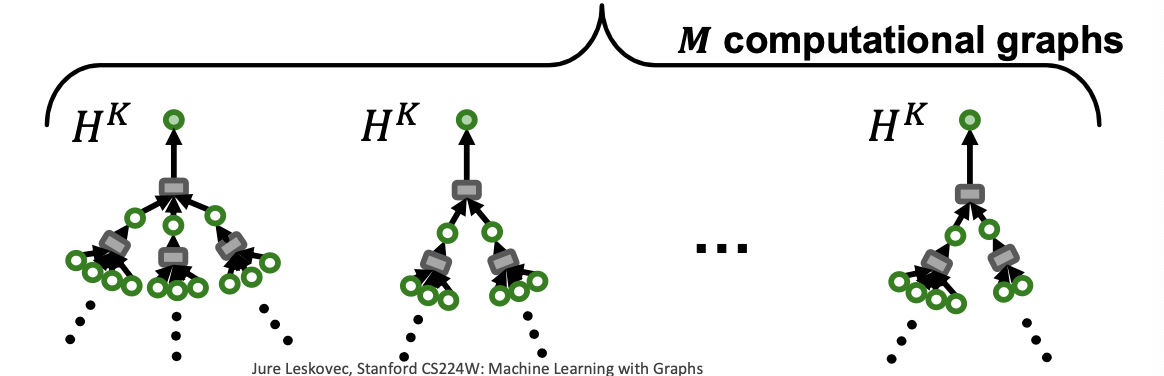
Computing Node Embeddings

• Key insight: To compute embedding of a single node, all we need is the $K$-hop neighborhood (which defines the computation graph)

• Given a set of $M$ different nodes in a mini-batch, we can generate their embeddings using $M$ computational graphs. Can be computed on GPU.

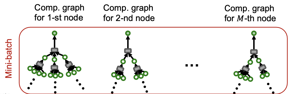
Stochastic Training of GNNs

• We can now consider the following SGD strategy for training $K$-layer GNNs:
  • Randomly sample $M(<<N)$ root nodes
  • For each sampled root node $v$:
    • Get $K$-hop neighborhood and construct the computation graph
    • Use the above to generate $v$’s embedding
  • Compute the loss $l_{sub}(\theta)$ averaged over the $M$ nodes
  • Perform SGD: $\theta \leftarrow \theta - \nabla l_{sub}(\theta)$

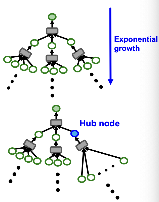
Issue with Stochastic Training

• For each node, we need to get the entire $K$-hop neighborhood and pass it through the computation graph

• We need to aggregate lot of information just to compute one node embedding

• Some computational redundancy

• $2^{nd}$ issue:
  • Computation graph becomes exponentially large with respect to the layer size $K$.
  • Computation graph explodes when it hits a hub node (high-degree node)

Neighborhood Sampling

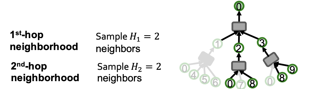
Key idea: Construct the computational graph by (randomly) sampling at most $H$ neighbors at each hop.

• Example $(H=2)$:

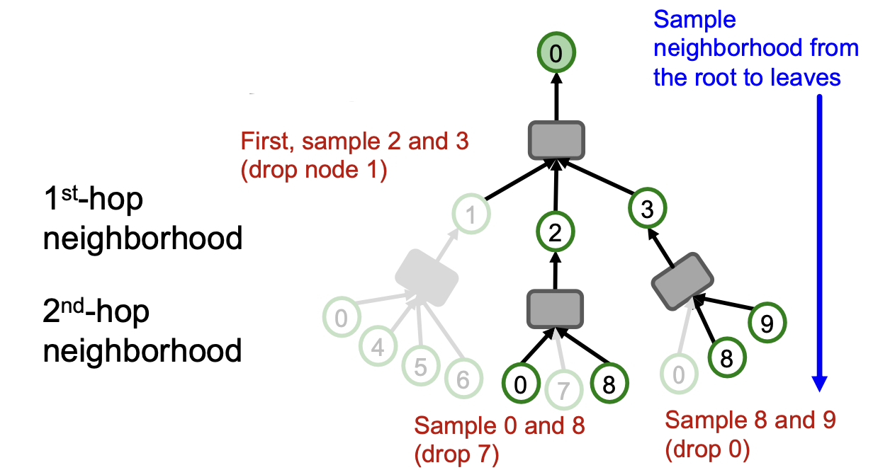
We can use the pruned computational graph to more efficiently compute node embeddings.(剪枝操作)

Neighborhood Sampling Algorithm

Neighbor sampling for $K$-layer GNN

• For $k = 1,2,\cdots,K$:
  • For each node in $k$-hop neighborhood:
  • (Randomly)sample at most $H_k$ neighbors:

  

• $K$-layer GNN will at most involve $\Pi_{k=1}^K H_k$ leaf nodes in computational graph

Remarks on Neighbor Sampling

• Remark 1: Trade-off in sampling number $H$
  • Smaller $H$ leads to more efficient neighbor aggregation, but results are less stable traning due to the large variance in neighbor aggregation

• Remark 2: Computational time
  • Even with neighbor sampling, the size of the computational graph is still exponential with respect to number of GNN layers $K$.
  • Adding one GNN layer would make computation $H$ times more expensive.

• Remark 3: How to sample the nodes
  • Random sampling: fast but many times not optimal (may sample many “unimportant” nodes)
  • Random Walk with Restarts:
    • Natural graphs are “scale free”, sampling random neighbors, samples many low degree “leaf” nodes.
    • Strategy to sample important nodes:
      • Compute Random Walk with Restarts score $R_i$ starting at the green node
      • At each level sample $H$ neighbors $i$ with the highest $R_i$

    

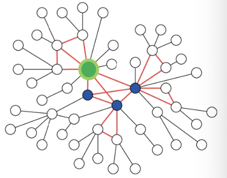
    • This strategy works much better in practice.

Scaling Up GNNs

Issues with Neighbor Sampling

• The size of computational graph becomes exponentially large w.r.t the #GNN layers

• Computation is redundant, especially when nodes in a mini-batch share many neighbors

Recall: Full Batch GNN

• In full-batch GNN implementation, all the node embeddings are updated together using embeddings of the previous layer.
  • In each layer, only $2^* \#$(edges) messages need to be computed.
  • For $K$-layer GNN, only $2K^*\#$(edges) messages need to be computed
  • GNN’s entire computation is only linear in #(edges) and #(GNN layers). Fast!

Update for all $v \in V$

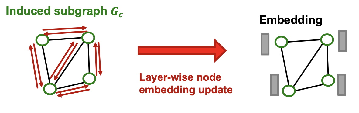
Insight from Full-batch GNN

• The layer-wise node embedding update allows the re-use of embeddings from the previous layer.

• This significantly reduces the computational redundancy of neighbor sampling.
  • Of course, the layer-wise update is not feasible for a large graph due to limited GPU memory.
    • Requires putting the entire graph and features on GPU.

Subgraph Sampling

• Key idea: We can sample a small subgraph of the large graph and then perform the efficient layer-wise node embeddings update over the subgraph

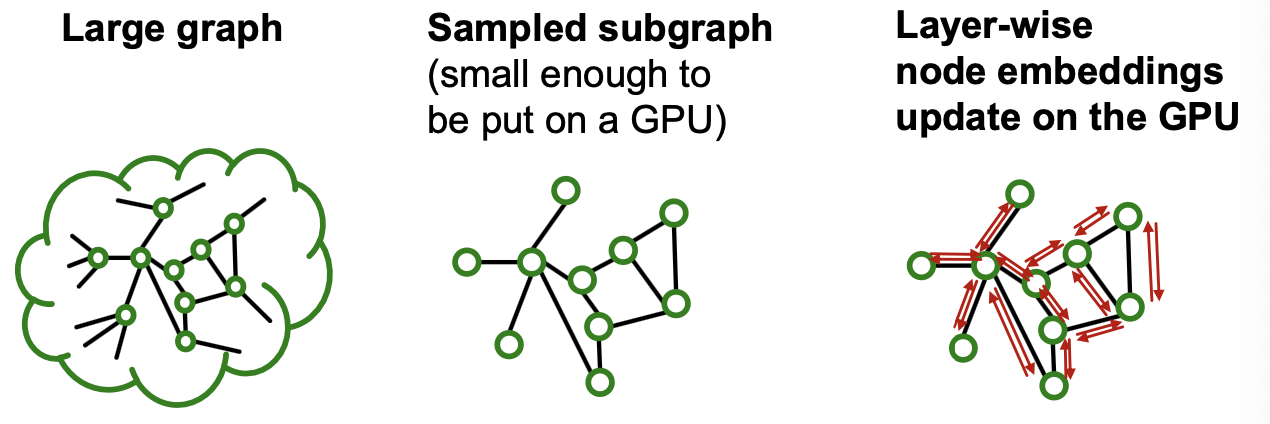
• Key question: What subgraphs are good for training GNNs
  • Recall: GNN performs node embedding by passing messages via the edges.
    • Subgraphs should retain edge connectivity structure of the original graph as much as possible.
    • This way, the GNN over the subgraph generates embeddings closer to the GNN over the original graph.

Subgraph Sampling: Case Study

• Which subgraph is good for training GNN?

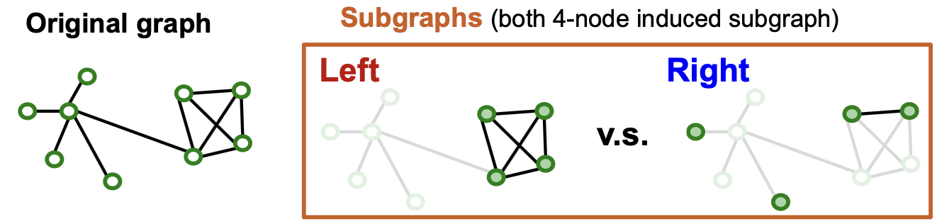
• Left subgraph retrains the essential community structure among the 4 nodes → Good

• Right subgraph drops many connectivity patterns, even leading to isolated nodes → Bad

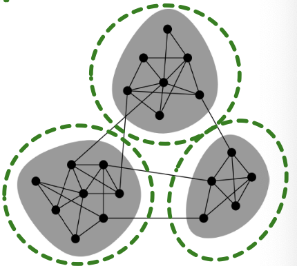
Exploiting Community Structure

Real-world graph exhibits community structure

• A large graph can be decomposed into many small communities

Key insight: Sample a community as a subgraph. Each subgraph retains essential local connectivity pattern of the original graph.

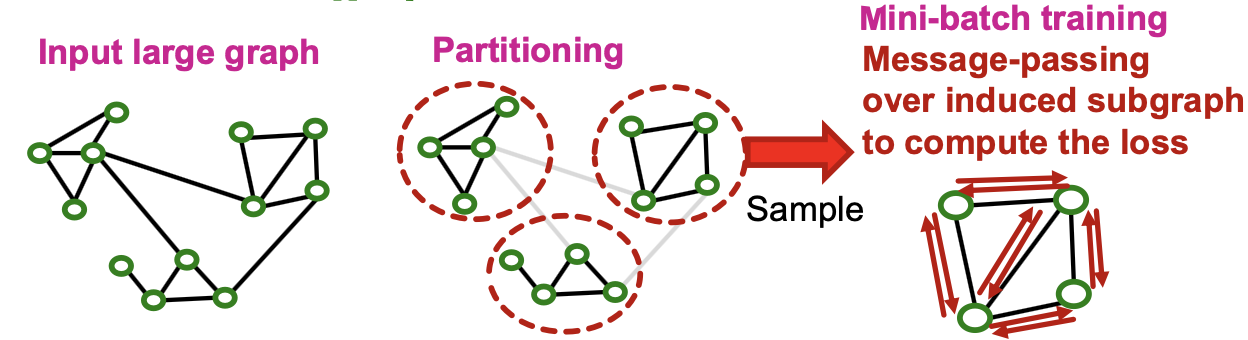
Cluster-GCN: Overview

• We first introduce “vanilla” Cluster-GCN

• Cluster-GCN consists of two steps:
  • Pre-processing: Given a large graph, partition it into groups of nodes (i.e., subgraphs).
  • Mini-batch training: Sample one node group at a time. Apply GNN’s message passing over the induced subgraph.

Cluster-GCN: Pre-processing

• Given a large graph $G=(V,E)$, partition its nodes $V$ into $C$ groups: $V_1,\cdots,V_C$
  • We can use any scalable community detection methods, e.g., Louvain, METIS [Karypis et al. SIAM 1998]

• $V_1,\cdots,V_C$ induces $C$ subgraphs, $G_1,\cdots,G_C$
  • Recall: $G_c = (V_c,E_c)$, where $E_c = \{(u,v)|u,v \in V_c\}$

  

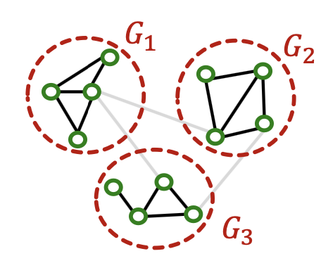
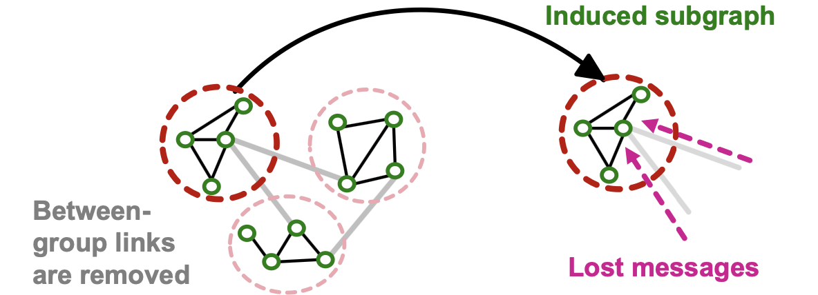
  Notice: Between-group edges are not included in $G_1,\cdots,G_C$.

Cluster-GCN: Mini-batch Training

• For each mini-batch, randomly sample a node group $V_c$.

• Construct induced subgraph $G_c = (V_c,E_c)$

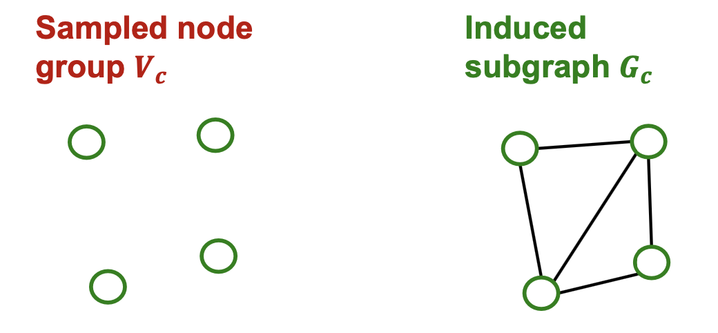
• Apply GNN’s layer-wise node update over $G_c$ to obtain embedding $h_v$ for each node $v \in V_c$.

• Compute the loss for each node $v \in V_c$ and take average:

• Update params: $\theta \leftarrow \theta - \nabla l_{sub}(\theta)$

Issues with Cluster-GCN

• The induced subgraph removes between-group links.

• As a result, messages from other groups will be lot during message passing, which could hurt the GNN’s performance

• Graph community detection algorithm puts similar nodes together in the same group.

• Sampled node group tends to only cover the small-concentrated portion of the entire data.

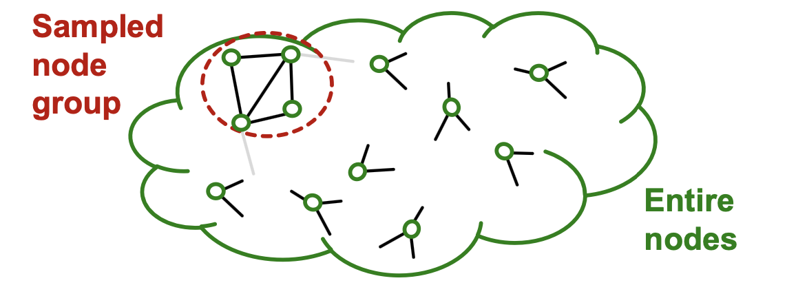
• Sampled nodes are not divers enough to be represent the entire graph structure:
  • As a result, the gradient averaged over the sampled nodes, $\frac{1}{|V_c|}\sum_{v\in V_c} l_v(\theta)$, becomes unreliable.
    • Fluctuates a lot from a node group to another.
    • In other words, the gradient has high variance.
  • Leads to slow convergence of SGD

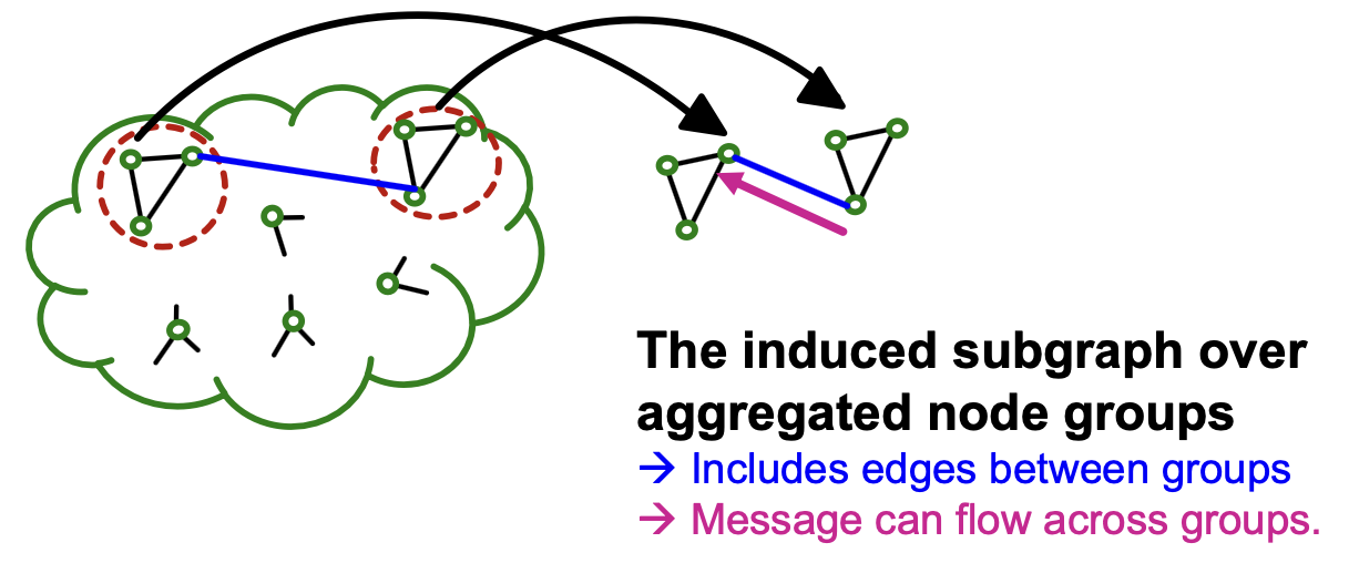
• Solution: Aggregate multiple node groups per mini-batch.

• Partition the graph into relatively-small groups of nodes.

• For each mini-batch:
  • Sample and aggregate multiple node groups.
  • Construct the induced subgraph of the aggregated node group.
  • The rest is the same as vanilla Cluster-GCN (compute node embeddings and the loss , update parameters)

• Why does the solution work?
  • Sampling multiple node groups
    • Makes the sampled nodes more representative of the entire nodes. Leads to less variance in gradient estimation.

    

Advanced Cluster-GCN

Similar to vanilla Cluster-GCN, advanced Cluster-GCN also follows a 2-step approach.

• 1) Pre-processing step:
  • Given a large graph $G = (V,E)$, partition its nodes $V$ into $C$ relatively-small groups: $V_1,V_2,V_3,\cdots,V_C$
    • $V_1,V_2,V_3,\cdots,V_C$ needs to be small so that even if multiple of them are aggregated, the resulting group would not be too large.

• 2) Mini-batch training:
  • For each mini-batch, randomly sample a set of $q$ node groups: $\{V_{t_1},\cdots,V_{t_q}\} \subset \{V_1,\cdots,V_C\}$.
  • Aggregate all nodes across the sampled node groups: $V_{aggr} = V_1 \cup V_2 \cdots \cup V_{t_q}$
  • Extract the induced subgraph $G_{aggr} = (V_{aagr},E_{aggr})$ where $E_{aagr} = \{(u,v)|u,v \in V_{aagr}\}$
    • $E_{aggr}$ also includes between-group edges!

Comparison of Time Complexity

• Generate $M(<<N)$ node embeddings using $K$ -layer GNN (N: #all nodes)

• Neighbor-sampling (sampling $H$ nodes per layer):
  • For each node, the size of $K$-layer computational graph is $H^K$.
  • For $M$ nodes, the cost is $M \cdot H^K$

  

• Cluster-GCN:
  • Perform message passing over a subgraph induced by the $M$ nodes.
  • The subgraph contains $M \cdot D_{avg}$ edges, where $D_{avg}$ is the average node degree.
  • K-layer message passing over the subgraph costs at most $K \cdot M \cdot D_{avg}$.

• In summary, the cost to generate embeddings for $M$ nodes using $K$-layer GNN is:
  • Neighbor-sampling (sample $H$ nodes per layer): $M \cdot H^K$
  • Cluster-GCN: $K\cdot M \cdot D_{avg}$

• Assume $H = D_{avg}/2$. In other words, $50\%$ of neighbors are sampled.
  • Then, Cluster-GCN (cost: $2MHK$) is much more efficient than neighbor sampling (cost: $MH^K$).
  • Linear (instead of exponential) dependency w.r.t. $K$.

Scaling up by Simplifying GNN Architecture

Roadmap of Simplifying GCN

• We start from Graph Convolutional Network (GCN)

• We simplify GCN(”SimplGCN”) by removing the non-linear activation from the GCN.
  • SimplGCN demonstrated that the performance on benchmark is not much lower by the simplification.
  • Simplified GCN turns out to be extremely scalable by the model design.
  • The simplification strategy is very similar to the one used by LightGCN for recommender systems.

Quick Overview of LightGCN

• Adjacency matrix: $A$

• Degree matrix: $D$

• Normalized adjacency matrix: $\tilde{A} = D^{-1/2}AD^{1/2}$

• Let $E^{(k)}$ be the embedding matrix at $k$-th layer.

• Let $E$ be the input embedding matrix.
  • We backprop into $E$.

• GCN’s aggregation in the matrix form
  • $E^{(k+1)} = ReLU (\tilde{A}E^{(k)}W^{(k)})$

• Removing ReLU non-linearity gives us
  • $E^{(K)} = \tilde{A}^{K}EW$, where $W = W^{(0)} \cdots W^{(K-1)}$
    • $\tilde{A}^{K}E$: Diffusing node embeddings along the graph.

• Efficient algorithm to obtain $\tilde{A}^KE$
  • Start from input embedding matrix $E$.
  • Apply $E \leftarrow \tilde{A}E$ for $K$ times.

• Weight matrix $W$ can be ignored for now.
  • $W$ acts as a linear classifier over the diffused node embeddings $\tilde{A}^KE$.

Differences to LightGCN

• SimplGCN adds self-loops to adjacency matrix $A$:
  • $A \leftarrow A+I$
    • Follows the original GCN by Kipf & Welling.

• SimplGCN assumes input node embeddings $E$ to be given as features:
  • Input embedding matrix $E$ is fixed rather than learned.
  • Important consequence: $\tilde{A}^KE$ needs to be calculated only once.
    • Can be treated as a pre-processing step.

Simplified GCN: “SimplGCN”

• Let $\tilde{E} = \tilde{A}^KE$ be pre-processed feature matrix.
  • Each row stores the pre-processed feature for each node.
  • $\tilde{E}$ can be used as input to any scalable ML models (e.g., linear model, MLP).

• SimplGCN empirically shows learning a linear model over $\tilde{E}$ often gives performance comparable to GCN!

Comparison with Other Methods

• Compared to neighbor sampling and cluster-GCN, SimplGCN is much more eddicient.
  • SimplGCN computes $\tilde{E}$ only once at the beginning.
    • The pre-processing (sparse matrix vector product,($E \leftarrow \tilde{A}E$) can be performed efficiently on CPU.
  • Once $\tilde{E}$ is obtained, getting an embedding for node $v$ only takes caonstant time!
    • Just look up a row for node $v$ in $\tilde{E}$.
    • No need to build a computational graph or sample a subgraph.

• But the model is less expressive.

Potential Issue of Simplified GCN

• Compared to the original GNN models, SimplGCN’s expressive power is limited due to the lack of non-linearity in generating node embeddings.

• Surprisingly, in semi-supervised node classification benchmark, SimplGCN works comparably to the original GNNs despite being less expressive.

Graph Homophily

• Many node classification tasks exhibit homophily structure, i.e., nodes connected by edges tend to share the same target labels.

When does Simplified GCN Work?

• Recall the preprocessing step of the simplified GCN: Do $E \leftarrow \tilde{A}E$ for $K$ times.
  • $E$ is node feature matrix $E=X$

• Pre-processed features are obtained by iteratively averaging their neighboring node features.

• As a result, nodes connected by edges tend to have similar pre-processed features.

• Premise: Model uses the pre-processed node features to make prediction.

• Nodes connected by edges tend to get similar pre-processed features.
  • Nodes connected by edges tend to be predicted the same labels by the model

• Simplified SGC’s prediction aligns well with the graph homophily in many node classification benchmark datesets.