CS224W-Machine Learning with Graph-GNN1

Basics of Deep Learning

Loss function:
- $f$ can be a simple linear layer, an MLP, or other neural networks (e.g., a GNN later)

\min_{\Theta} \mathcal{L}(\mathcal{y},f_{\Theta}(x))

Simple a minibatch of input $x$ .

Forward propagation: Compute $\mathcal{L}$ given $x$

Back-propagation: Obtain gradient $\nabla_{\Theta}\mathcal{L}$ using a chain rule.

Use stochastic gradient descent (SGD) to optimize $\mathcal{L}$ for $\Theta$ over many iterations.

Deep Learning for Graphs

Setup

Graph $G$ .

$V$ is the vertex set

$A$ is the adjacency matrix (assume binary)

$X \in \mathbb{R}^{|V| \times m}$ is a matrix of node features

$v$ : a node in $V$ ; $N(v)$ : the set of neighbors of $v.$

Node Features:
- Social networks: Use profile, User image
- Biological networks: Gene expression profiles, gene functional information
- When there is node feature in the graph dataset:
  - Indicator vectors (one-hot encoding of a node)
  - Vector of constant 1: $[1,1,\cdots,1]$

A Naive Approach

Join adjacency matrix and features

Feed them into a deep neural net

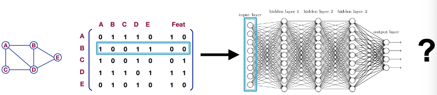
Issues with this idea:
- $O(|V|)$ parameters
- Not applicable to graphs of different sizes
- Sensitive to node ordering

Convolutional Networks (卷积网络)

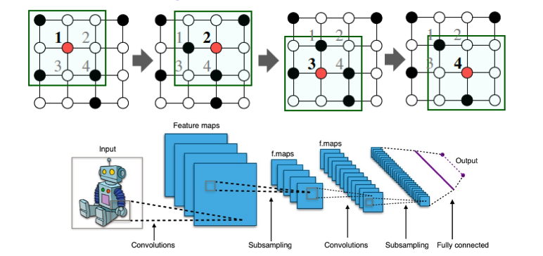
Goal is to generalize convolutions beyond simple lattices Leverage node features/attributes(e.g., text, images)

Real-World Graphs

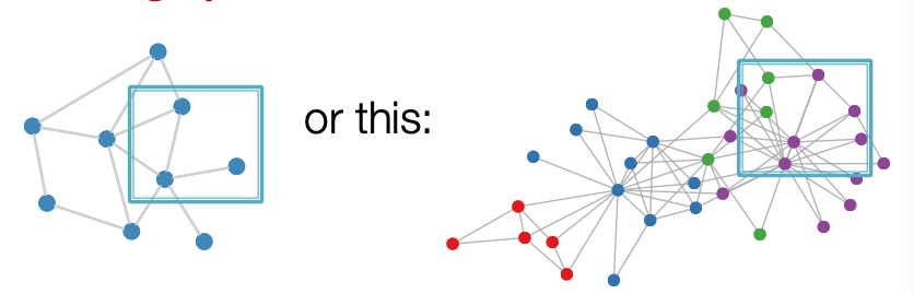
There is no fixed notion of locality or sliding window on the graph

Graph is permutation invariant

Permutation Invariance (排列不变性)

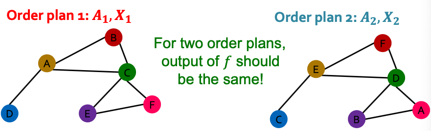
Graph does not have a canonical order of the nodes!

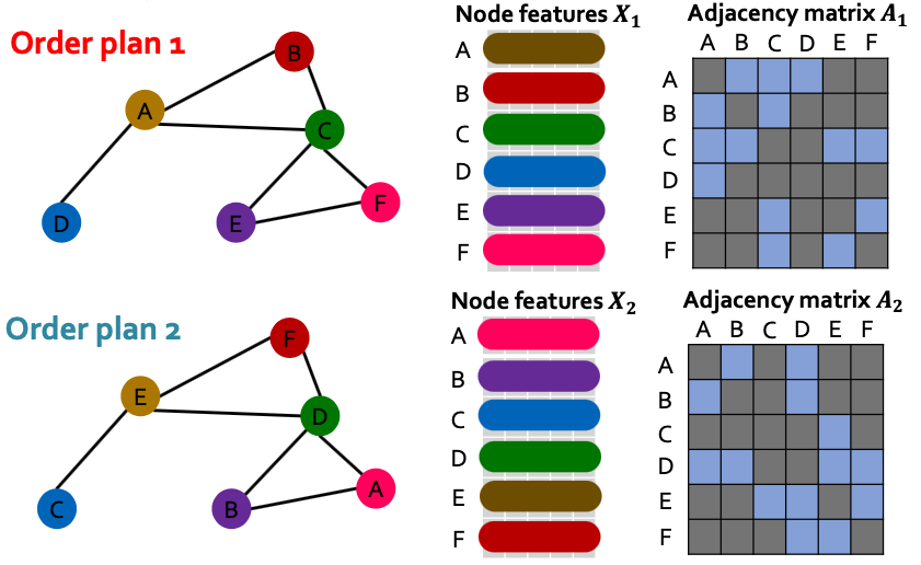
We can have many different order plans.

What does it mean by “graph representation” is same for two order plans?

Consider we learn a function $f$ that maps a graph $G = (A,X)$ to a vector $\mathbb{R}^d$ then
- In other words, $f$ maps a graph to a $d-dim$ embedding
- $A$ is the adjacency matrix
- $X$ is the node feature matrix

f(A_1,X_1) = f (A_2,X_2)

Then, if $f(A_i,X_i) = f(A_j,X_j)$ for any order plan $i$ and $j$ , we formally say $f$ is a permutation invariant function.
- For a graph with $\lvert V\rvert$ nodes, there are $\lvert V \rvert!$ different order plans. (排列组合)

Definition: For any graph function $f:\mathbb{R}^{|V| \times m} \times \mathbb{R}^{|V| \times |V|} \rightarrow \mathbb{R}^d$ , $f$ is permutation-invariant if $f(A,X) = f(PAP^T,PX)$ for any permutation $P$ .
- $m$ : each node has a $m-dim$ feature vector associated with it.
- $d$ : output embedding dimensionality of embedding the graph $G = (A,X)$
- Permutation $P$ : a shuffle of the node order. Expamle: $(A,B,C) \rightarrow (B,C,A)$

Permutation Equivariance

For node representation: We learn a function $f$ that maps nodes of $G$ to a matrix $\mathbb{R}^{|V| \times d}$
- In other words, each node in $V$ is mapped to a $d-dim$ embedding.

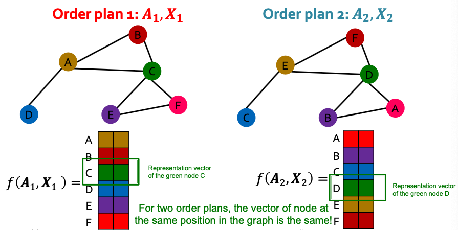
If the output vector of a node at the same position in the graph remains unchanged for any order plan, we say $f$ is permutation equivariant.

Definition: For any node function $f:\mathbb{R}^{|V| \times m} \times \mathbb{R}^{|V|\times|V|} \rightarrow \mathbb{R}^{|V|\times d}$ , $f$ is permutation-equivariant if $P f(A,X) = f(PAP^T,PX)$ for any permutation $P$ .
- $m$ : each node has a $m-dim$ feature vector associated with it
- $f$ maps each node in $V$ to a $d-dim$ embedding.

Summary: Invariance and Equivariance

Permutation-invariant(Permute the input, the output stays the same)

f(A,X) = f(PAP^T,PX)

Permutation-equivariant(Permute the input, output also permutes accordingly)

Pf(A,X) = f(PAP^T,PX)

Examples:
- $f(A,X) = 1^TX$ Permutation-invariant
  - $f(PAP^T,PX) = 1^TPX = 1^TX = f(A,X)$
- $f(A,X) = AX$ Permutation-equivariant
  - $f(PAP^T,PX) = PAP^TPX = PAX = Pf(A,X)$

Graph Convolutional Networks [Kipf and Welling, ICLR 2017]

图卷积网络

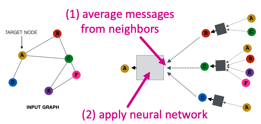
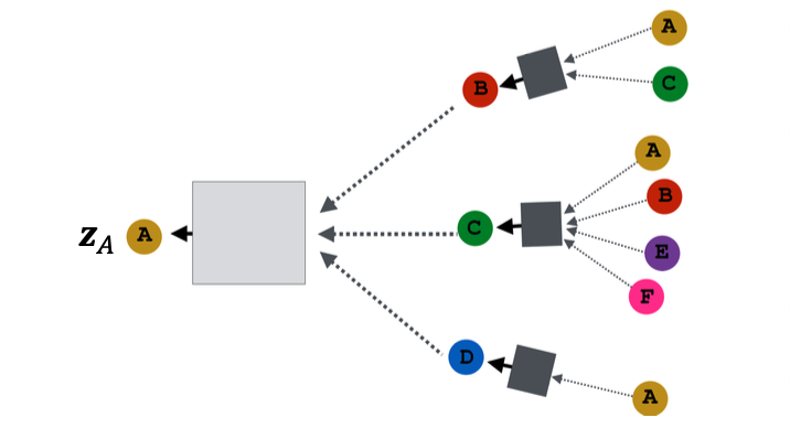
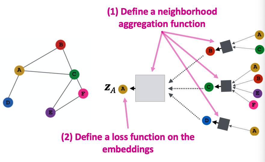
Idea: Node’s neighborhood defines a computation graph

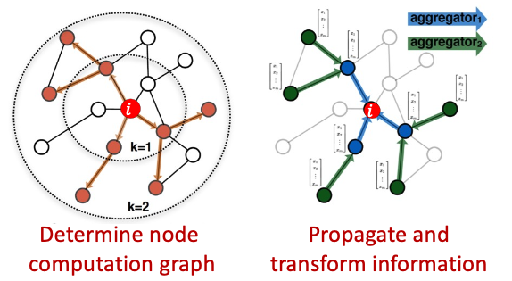
How to propagate information across the graph to compute node features?

Key idea: Generate node embeddings based on local network neighborhoods

Nodes aggregate information from their neighbors using neural networks (上图)

Network neighborhood defines a computation graph (下图)

Deep Model: Many Layers

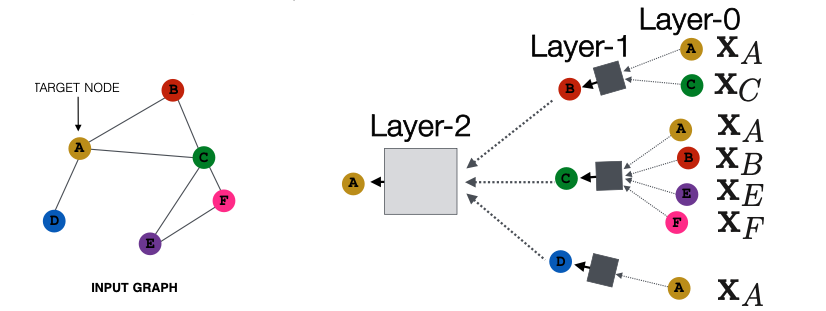
Model can be of arbitrary depth:

Nodes have embeddings at each layer

Layer-0 embedding of node $v$ is its input feature, $x_v$

Layer-k embedding gets information from nodes that are $k$ hops away

Neighborhood Aggregation (邻居节点的聚合)

Key distinctions are in how different approaches aggregate information across the layers

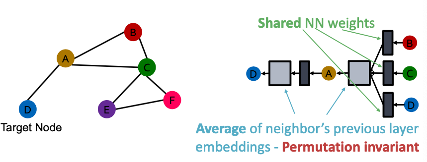
Basic approach: Average information from neighbors and apply a neural network.

h_v^0 = \textbf{x}_v

Initial 0-th layer embeddings are equal to node features

h_v^{(k+1)} = \sigma(W_k \sum_{u \in N(v)} \frac{h_u^{(k)}}{|N(v)|}+B_k h_v^{(u)}),\ \forall k \in \{0,\cdots,K-1\}

$\sigma()$ : Non-linearity (e.g., ReLU)

$\sum_{u \in N(v)} \frac{h_u^(k)}{|N(v)|}$ : Average of neighbor’s previous layer embeddings

$h_v^{(k)}$ : embedding og $v$ at layer $k$ .

$K$ : total number of layers

\textbf{z}_v = h_v^{(K)}

$\textbf{z}_v$ : Embedding after $K$ layers of neighborhood aggregation

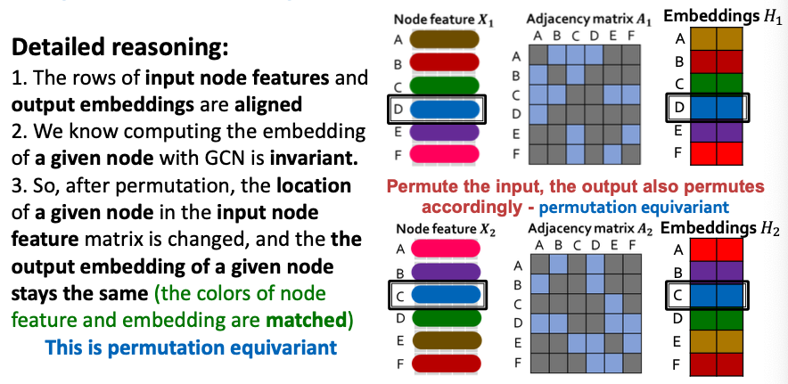
GCN: Invariance and Equivariance

Invariance and Equivariance Properties for a GCN?

Given a node, the GCN that computes its embedding is permutation invariant

Considering all nodes in a graph, GCN computation is permutation equivariant

How do we train the GCN to generate embeddings?

Need to define a loss function on the embeddings.

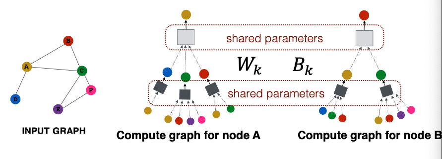
Model Parameters

h^{(0)}_v = \textbf{x}_v

h_v^{(k+1)} = \sigma(W_k \sum_{u \in N(v)} \frac{h_u^{(k)}}{|N(v)|}+B_k h_v^{(u)}),\ \forall k \in \{0,\cdots,K-1\}

\textbf{z}_v = h^{(K)}_v

$W_k,B_k$ are trainable weight matrices.

$h_v^k$ : the hidden representation of node $v$ at layer $k$ .

$W_k$ : weight matrix for neighborhood aggregation

$B_k$ : weight matrix for transforming hidden vector of self.

Matrix Formulation

Many aggregations can be performed efficiently by (spare) matrix operations

Let $H^{(k)} = [h_1^{(k)},\cdots,h_{|V|}^{(k)}]^T$

Then: $\sum_{u \in N_v}h^{(k)}_u = A_{v,:}H^{(k)}$

Let $D$ be diagonal matrix where $D_{v,v} = Deg(v) = |N(v)|$
- The inverse of $D$ : $D^{-1}$ is also diagonal: $D^{-1}_{v,v} = \frac{1}{|N(v)|}$

Therefore,

\sum_{u \in N(v)} \frac{h_u^{(k-1)}}{|N(v)|} \Longrightarrow H^{(k+1)} = D^{-1}AH^{(k)}

Re-writing update function in matrix form:
$H^{(k+1)} = \sigma (\widetilde{A}H^{(k)}W^T_k + H^{(k)}B^T_k)$
where $\widetilde{A} = D^{-1}A$
- $\widetilde{A}H^{(k)}W_k^T$ : neighborhood aggregation
- $H^{(k)}B_k^T$ : self transformation

在真实情况下，可以用于稀疏矩阵(spare matrix)

Train A GNN

Node embedding $\textbf{z}_v$ is a function of input graph.

Supervised setting: We want to minimize loss $\mathcal{L}$ :
$\min_{\Theta} \mathcal{L}(\textbf{y},f_{\Theta}(\textbf{z}_v))$
- $\textbf{y}$ : node label
- $\mathcal{L}$ could be $L_2$ if $\textbf{y}$ is real number, or cross entopy if $\textbf{y}$ is categorical

Unsupervised setting:
- No node label available
- Use the graph structure as the supervision!

Unsupervised Training (无监督训练)

“类似的”节点有着相似的嵌入
- where $y_{u,v} =1$ when node $u$ and $v$ are similar
- $\textbf{z}_u = f_{\Theta}(u)$ and $DEC(\cdot,\cdot)$ is the dot product

\min_{\Theta}\mathcal{L} = \sum_{\textbf{z}_u,\textbf{z}_v} CE(y_{u,v},DEC(\textbf{z}_u,\textbf{z}_v))

CE is the cross entropy loss:
- $CE(\textbf{y},f(\textbf{x})) = - \sum_{i=1}^C (y_i \log f_{\Theta}(x)_i)$
  - $y_i$ and $f_{\Theta}(x)_i$ are the actual and predicted values of the $i$ -th class.
  - Intuition: the lower the loss, the closer the prediction is to one-hot.

Node similarity can be anything from Random walks or Matrix factorization

Supervised Training (监督训练)

Directly train the model for a supervised task (e.g. node classification)

Use cross entropy loss

\mathcal{L} = - \sum_{v \in V} \textbf{y}_v \log (\sigma(\textbf{z}^T_v\theta))+ (1-\textbf{y}_v)\log (1-\sigma(\textbf{z}^T_v \theta))

$\textbf{y}_v$ : Node class label

$\textbf{z}_v^T$ : Encoder output: node embedding

$\theta$ : Classification weights

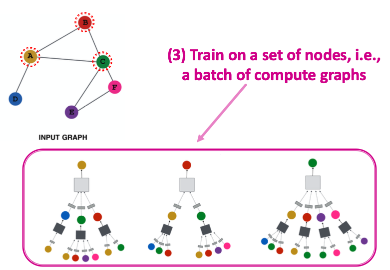
Model Design: Overview

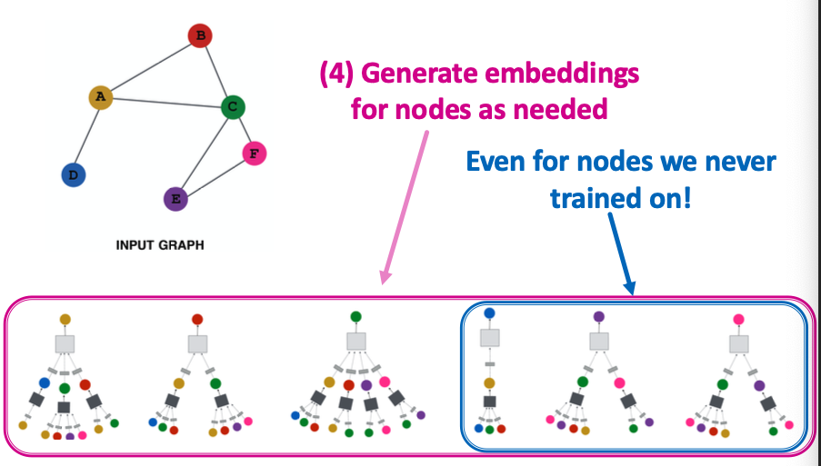
Inductive Capability (归纳)

The same aggregation parameters are shared for all nodes:

The number of model parameters is sublinear in $|V|$ and we can generalize to unseen nodes!

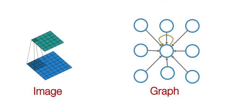
GNNs subsume CNNs

GNN CNN Transformer

Convolutional Neural Network

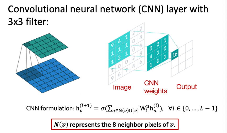
CNN vs. CNN

GNN formulation:

h_v^{(l+1)} = \sigma (W_l \sum_{u \in N(v)} \frac{h_u^{(l)}}{|N(v)|} + B_l h_v^{(l)}), \ \forall l \in \{0,\cdots,L-1\}

CNN formulation: (previous slide)

h_v^{(l+1)} = \sigma (\sum_{u \in N(v)}W_l^u h_u^{(l)} + B_l h_v^{(l)}), \ \forall l \in \{0,\cdots,L-1\}

Key difference: We can learn different $W_l^u$ for different “neighbor” $u$ for pixel $v$ on the image. The reason is we can pick an order for the $9$ neighbors using relative position to the center pixel: $\{(-1,-1),(-1,0),\cdots,(1,1)\}$

Transformer

Key component: Self-attention

Every token/word attends to all the other tokens/words via matrix calculation.

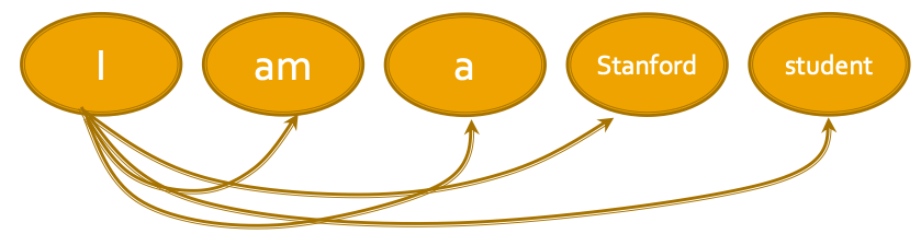
Definition: A general definition of attention: Given a set of vector values, and a vector query, attention is a technique to compute a weighted sum of the values, dependent on the query.

Transformer layer can be seen as a special GNN that runs on a fully connected “word” graph!