CS224W-Machine Learning with Graph-GNN2
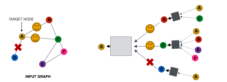
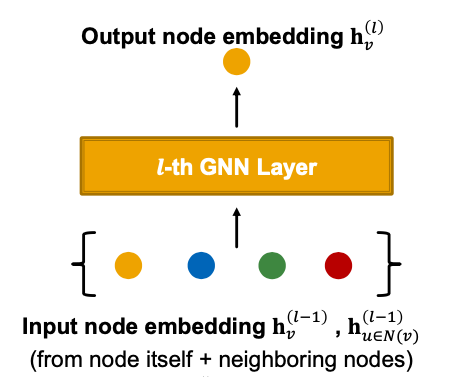
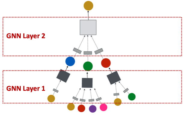
A Single Layer of a GNN
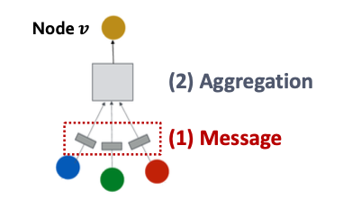
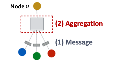
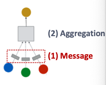
A GNN Layer = Message + Aggregation
- Different instantiations under this perspective
- GCN, GGraphSAGGE, GAT,…

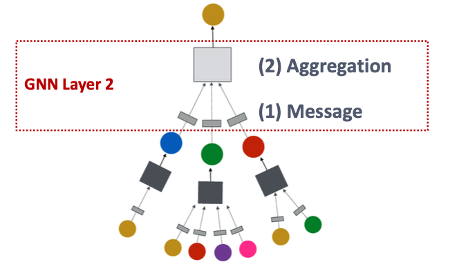
Compress a set of vectors into a single vector
Message Computation (消息计算)
- Message function:
- : 消息计算时的权重/函数
- Intuition: Each node will create a message, which will be sent to other nodes later.
- Example: A Linear layer
- Multiply node features with weight matrix
Message Aggregation (消息聚合)
- Aggregation function:
- : 聚合器
- Intuition: Node will aggregate the messages from its neighbors
- Example: or aggregator
-
Message Aggregation: Issue (考虑在聚合时可能会出现自身节点信息的丢失,即自己到自己时的信息可能会发生丢失)
Issue: Information from node itself could get lost
- Computation of does not directly depend on
Solution: Include when computing
- Message: compute message from node itself
- Usually, a different message computation will be performed
- 在不同的连接节点的时候使用不同的函数/权重
- Usually, a different message computation will be performed
- Aggregation: After aggregating from neighbors, we can aggregate the message from node itself
- Via concatenation or summation
- First aggregate from neighbors
- Then aggregate from node itself
Classical GNN Layers
GCN Graph Convolutional Networks
- Message
- Each neighbor: . Normalized by node degree
- Aggregation:
- Sum over message from neighbors, then apply activation
-
GraphSAGE
- Message is computed within the
- Two-stage aggregation
- Stage 1: Aggregation from node neighbors
- Stage 2: Further aggregate over the node itself
- Stage 1: Aggregation from node neighbors
GraphSAGE Neighbor Aggregation (GraphSAGE 邻居节点的聚合方法)
- Mean: Take a weighted average of neighbors
- Pool: Transform neighbor vectors and apply symmetric vector function or
- LSTM: Apply LSTM to reshuffled of neighbors
GraphSAGE: Normalization (在嵌入之后进行归一化)
Normalization
- Optimal: Apply normalization to at every layer
- , where (-norm)
- Without normalization, the embedding vectors have different scales (-norm) for vectors
- In some cases (not always), normalization of embedding results in performance improvement
- After normalization, all vectors will have the same -norm
Graph Attention Networks
- In GCN/GraphSAGE
- is the weighting factor (importance) of node ’s message to node .
- is defined explicitly based on the structural properties of the graph (node degree)
- All neighbors are equally important to node
根据这个权重,那就需要考虑加入注意力机制,即考虑到每个节点对本节点影响的程度不同,因此可以考虑加入注意力机制。
Not all node’s neighbors are equally important
- Attention is inspired by cognitive attention
- The attention focuses on the important parts of the input data and fades out the rest
- Idea: the NN should devote more computing power on that small but important part of the data.
- Which part of the data is more important depends on the context and is learned through training
Weighting factors be learned?
Goal: Specify arbitrary importance to different neighbors of each node in the graph
Idea: Compute embedding of each node in the graph following an attention strategy
- Nodes attend over their neighborhood’s message
- Implicitly specifying different weights to different nodes in a neighborhood
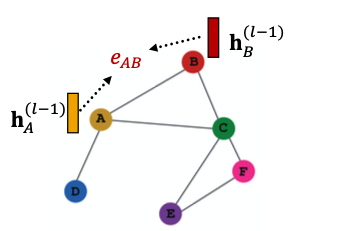
Attention Mechanism
Let be computed as a byproduct of an attention mechanism :
- Let a compute attention coefficients across pairs of nodes based on their messages:
- indicates the importance of ’s message to node
-
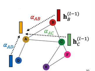
- Normalize into the final attention weight
- Use the softmax function, so that
- Weighted sum based on the final attention weight
Weighted sum using :
注意力机制 的形式?
Use a simple single-layer neural network have trainable paremeters (weights in the Linear layer)

- Parameters of are trained jointly
- Learn the parameters together with weight matrices(i.e., other parameter of the neural net ) in an end-to-end fashion
多头注意力机制(Multi-head Attention)
Stabilizes the learning process of attention mechanism
- Create multiple attention scores (each replica with a different set of parameters):
-
-
-
- Outputs are aggregated
- By concatenation or summation
-
Benefits of Attention Mechanism 注意力机制的好处
- Key benefit: Allows for (implicitly) specifying different importance values () to different neighbors
GNN Layers in Practice

Many modern deep learning modules can be incorporated into a GNN layer
- Batch Normalization
- Stabilize neural network training
- Dropout
- Prevent overfitting
- Attention/Gating
- Control the importance of a message
- More
- Any other useful deep learning modules
Batch Normalization
- Goal: Stabilize neural networks training
- Idea: Given a batch of inputs (node embeddings)
- Re-center the node embeddings into zero mean
- Re-scale the variance into unit variance
Setup
Input:
- node embeddings
Trainable Parameters:
Output:
- Normalized node embeddings
Step 1: Compute the mean and variance over embeddings
Step 2: Normalize the feature using computed mean and variance
Dropout

- Goal: Regullarize a neural net to prevent overfitting
- Idea:
- During training: with some probability , randomly set neurons to zero (turn off)
- During testing: Use all the neurons for computation
- Dropout for GNNs
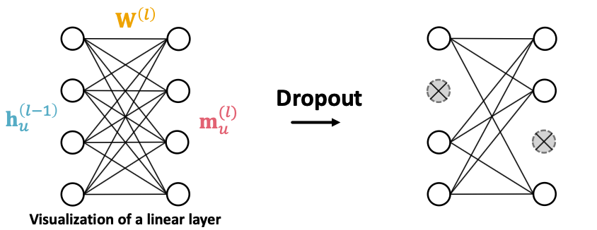
- In GNN, Dropout is applied to the linear layer in the message function
- A simple message function with linear layer:
- In GNN, Dropout is applied to the linear layer in the message function
Activation (non-linearity)
Apply activation to -th dimension of embedding
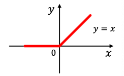
- Rectified linear unit (ReLU)
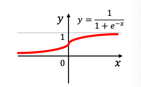
- Sigmoid
- Used only when we want to restrict the range of our embeddings
- Parametric ReLU
- Empirically performs better than ReLU
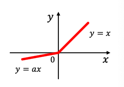
is a trainable parameter.
Stacking Layers of a GNN
- Stack layers sequentially
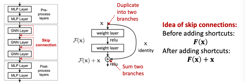
- Ways of adding skip connections
Construct a Graph Neural Network
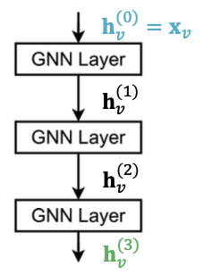
- The standard way: Stack GNN layers sequentially
- Input: Initial raw node feature
- Output: Node embeddings after GNN layers
如果GNN的层数过多会引起过于平滑的问题(Why?)
The Over-smoothing Problem
- the issue of stacking many GNN layer
- GNN suffers from the over-smoothing problem
- The over-smoothing problem: All the node embeddings converge to the same value
- This is bad because we want to use node embeddings to differentiate nodes
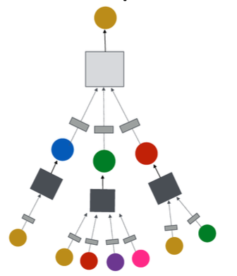
Receptive Field of a GNN
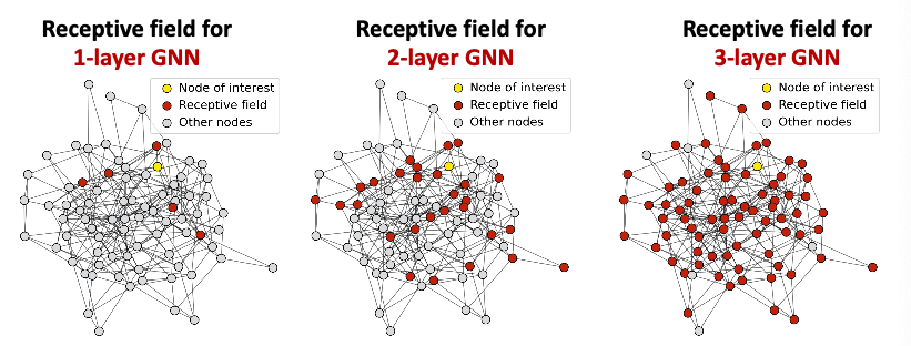
Receptive field: the set of nodes that determine the embedding of a node of interest
- In a -layer GNN, each node has a receptive field of -hop neighborhood
Receptive field overlap for two nodes
- The shared neighbors quickly grows when we increase the number of hops(num of GNN layers)
Via the notion of the receptive filed to explain over-smoothing
- We know the embedding of a node is determined by its receptive field
- If two nodes have highly-overlapped receptive fields, then their embeddings are highly similar
- Stack many GNN layers nodes will have highly-overlapped receptive fields node embeddings will be highly similar suffer from the over-smoothing problem.
层数过多之后,链接的节点越多,即扩展的节点越多,导致节点的嵌入就会越来越相似。都是连接的差不多的节点。
Be cautious when adding GNN layers - Unlike neural networks in other domains (CNN for image classification), adding more GNN layers do not always help.
Expressive Power for Shallow GNNs? How to make a shallow GNN more expressive?
- Solution 1: Increase the expressive power within each GNN layer
- In our previous examples, each transformation or aggregation function only include one linear layer
- We can make aggregation / transformation become a deep neural network!
- Solution 2: Add layers that do not pass messages
- A GNN does not necessarily only contain GNN layers
- add MLP layers (applied to each nodes)before and after GNN layers, as pre-process layers and post-process layers
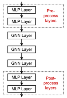
- A GNN does not necessarily only contain GNN layers
Pre-processing layers: Important when encoding node features is necessary.
Post-processing layers: Important when reasoning/ transformation over node embeddings are needed
If our problem still requires many GNN layers, we need to add skip connections in GNNs
- Add skip connections in GNNs
- Observation from over-smoothing: Node embeddings in earlier GNN layers can sometimes better differentiate nodes
- Solution: We can increase the impact of earlier layers on the final node embeddings, by adding shortcuts in GNN
为什么skip connections?
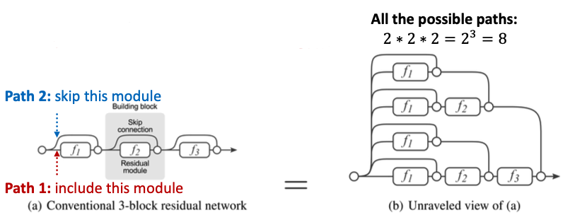
- Intuition: Skip connections create a mixture of models
- skip connections possible paths
- Each path could have up to modules
- We automatically get a mixture of shallow GNNs and deep GNNs
Example: GCN with Skip Connections
A standard GCN layer
A GCN layer with skip connection
Example: Other Options of Skip Connections
Directly skip to the last layer - The final layer directly aggregates from the all the node embeddings in the previous layers.
Graph Manipulation in GNNs
Idea: Raw input graph computational graph
- Graph feature augmentation
- Graph structure manipulation
Why Manipulate Graphs?
Our assumption so far has been: Raw input graph Computational graph
Reasons for breaking this assumption Graph Manipulation Approaches
- Feature level:
- The input graph lacks features Feature augmentation
- Structure level:
- The graph is too spare inefficient message passing Add virtual nodes/ edges
- The graph is too dense message passing is too costly Sample neighbors when doing message passing
- The graph is too large can not fit the computational graph into a GPU Sample subgraphs to compute embeddings
Feature Augmentation on Graphs
Why do we need feature augmentation?
Input graph does not have node features
- This is common when we only have the adj. matrix (邻接矩阵)
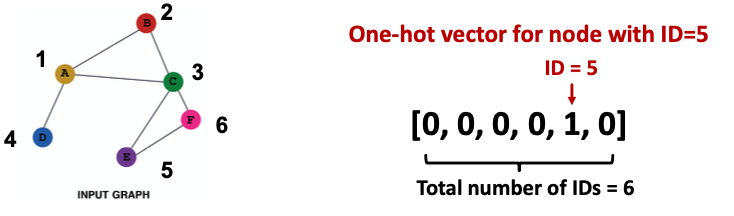
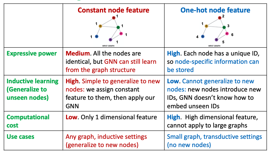
Standard approaches:
Assign constant values to nodes

Assign unique IDs to nodes
These IDs are converted into one-hot vectors
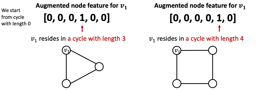
Certain structures are hard to learn by GNN
We can use cycle count as augmented node features
Other commonly used augmented features
- Clustering coefficient
- PageRank
- Centrality
-
Add Virtual Nodes/ Edges
Motivation: Augment sparse graphs
- Add virtual edges
- Common approach: Connect 2-hop neghbors via virtual edges
- Intuition: Instead of using adj. matrix for GNN computation, use
Example: Bipartite graphs
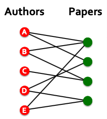
- Author-to-papers (they authored)
- 2-hop virtual edges make an author-author collaboration graph
- Add virtual nodes
- The virtual node will connect to all the nodes in the graph
- Suppose in a sparse graph, two nodes have shortest path distance of 10
- After adding the virtual node, all the nodes will have a distance of 2
- Node A - Virtual node - Node B
- Benefits: Greatly improves message passing in sparse graphs
- The virtual node will connect to all the nodes in the graph
- Our approach so far: All the neighbors are used for message passing
- Problem: Dense/large graphs, high-degree nodes
- New idea: (Randomly) determine a node’s neighborhood for message passing
Example: Neighborhood Sampling (类似于随机采样)
- For example, we can randomly choose 2 neighbors to pass messages
- Only nodes B and D will pass message to A
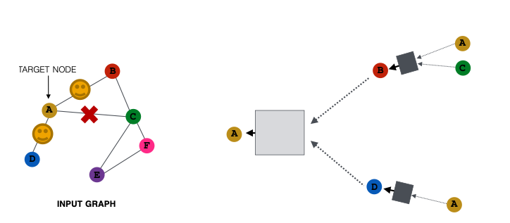
- Next time when we compute the embeddings, we can sample different neighbors
- Only nodes C and D will pass message to A
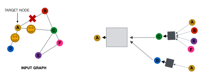
- In expectation, we can get embeddings similar to the case where all the neighbors are used
- Benefits: Greatly reduce computational cost