CS224W-Machine Learning with Graph-GNN3

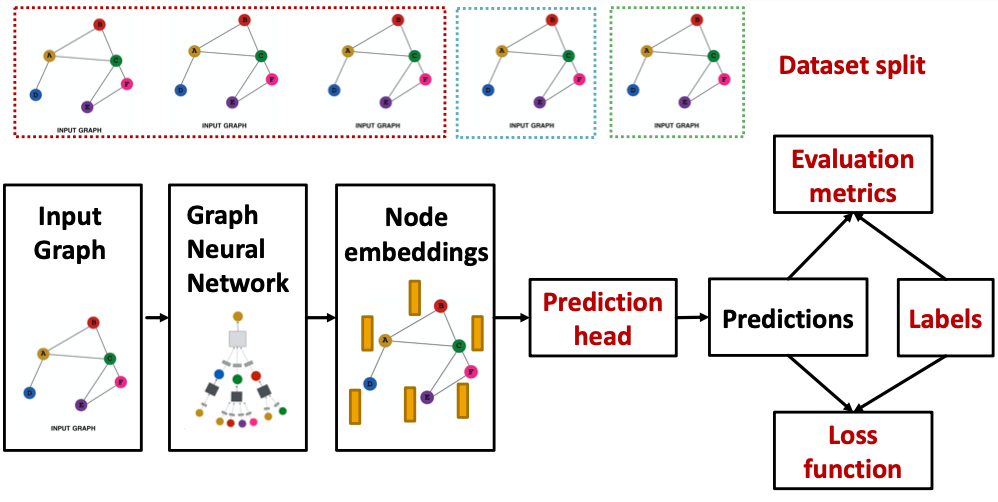
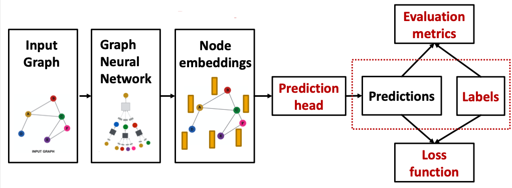
GNN Training Pipeline

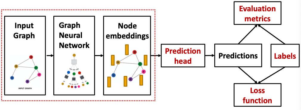
Output of a GNN: set of node embeddings $\{ \textbf{h}^{(L)}_v , \ \forall v \in G \}$

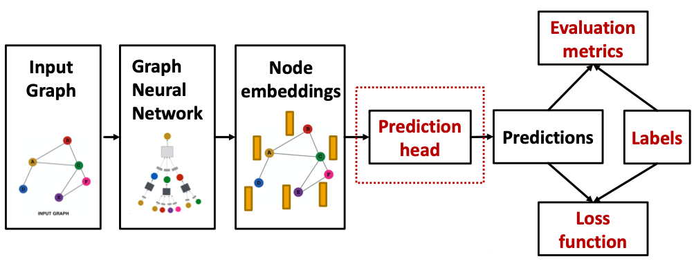
Different prediction heads: (Idea: Different task levels require different prediction heads)

Node-level tasks

Edge-level tasks

Graph-level tasks

Prediction Heads: Node-level

Node-level prediction: We can directly make prediction using node embeddings!

After GNN computation, we have $d$ -dim node embeddings: $\{ \textbf{h}^{(L)}_v\in \mathbb{R}^d, \forall \in G\}$

Suppose we want to make $k$ -way prediction
- Classification: classify among $k$ categories
- Regression: regress on $k$ targets

$\hat{\textbf{y}}_v = \text{Head}_{node} ( \textbf{h}^{(L)}_v) = \textbf{W}^{(H)} \textbf{h}_v^{(L)}$
- $\textbf{W}^{(H) } \in \mathbb{R}^{k \times d}$ : We map node embeddings from $\textbf{h}_{v}^{(L)} \in \mathbb{R}^d$ to $\hat{\textbf{y}}_v \in \mathbb{R}^k$ so that we can compute the loss.

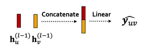
Prediction Heads: Edge-level

Edge-level prediction: Make prediction using pairs of node embeddings

Suppose we want to make $k$ -way prediction

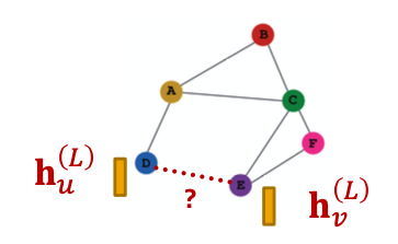
$\hat{\textbf{y}}_{uv} = \text{Head}_{edge}(\textbf{h}_u^{(L)},\textbf{h}_v^{(L)})$

\text{Options for } \ \text{Head}_{edge}( \textbf{h}_u^{(L)},\textbf{h}_v^{(L)})

Concatenation + Linear
- We have seen this is graph attention
- $\hat{\textbf{y}}_{uv} = \text{Linear}(\text{Concat}(\textbf{h}_u^{(L)}, \textbf{h}_v^{(L)}))$
- Here $\text{Linear}(\cdot)$ will map $2d$ -dimensional embeddings (since we concatenated embeddings) to $k$ -dim embeddings ( $k$ -way prediction)

Dot product
- $\hat{\text{y}}_{uv} = (\textbf{h}_u^{(L)})^T \textbf{h}_v^{(L)}$
- This approach only applies to $1$ -way prediction
- Applying to $k$ -way prediction:
  - Similar to multi-head attention: $\textbf{W}^{(1)}, \cdots,\textbf{W}^{(k)}$ trainable
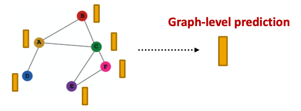
  $\begin{align*} \hat{y}_{uv}^{(1)} &= (\textbf{h}_u^{(L)})^T \textbf{W}^{(1)} \textbf{h}_v^{(L)}\\ &\cdots\\ \hat{y}_{uv}^{(k)} &= (\textbf{h}_u^{(L)})^T \textbf{W}^{(k)} \textbf{h}_v^{(L)} \\ \hat{y}_{uv} & = \text{Concat}(\hat{y}_{uv}^{(1)},\cdots,\textbf{y}_{uv}^{(k)}) \in \mathbb{R}^k \end{align*}$

Prediction Heads: Graph-level

Graph-level prediction: Make prediction using all the node embeddings in our graph

Suppose we want to make $k$ -way prediction

$\hat{y}_G = \text{Head}_{graph}(\{ \textbf{h}_v^{(L) \in \mathbb{R}^d }, \ \forall v \in G\})$

$\text{Head}_{graph}(\cdot)$ is similar to $\text{AGG}(\cdot)$ in a GNN layer!

\text{Options for} \ \text{Head}_{graph}(\{ \textbf{h}_v^{(L)} \in \mathbb{R}^d, \ \forall v \in G\})

Global mean pooling
$\hat{y}_G = \text{Mean}(\{ \textbf{h}_v^{(L)} \in \mathbb{R}^d, \ \forall v \in G\})$

Global max pooling
$\hat{y}_G = \text{Max}(\{ \textbf{h}_v^{(L)} \in \mathbb{R}^d, \ \forall v \in G\})$

Global sum pooling

\hat{y}_G = \text{Sum}(\{ \textbf{h}_v^{(L)} \in \mathbb{R}^d, \ \forall v \in G\})

Where does ground-truth come form?

Supervised Labels

Unsupervised Signals

\text{Supervised vs Unsupervised}

Supervised learning on graphs

Labels come form external sources (predict drug likeness of a molecular graph)

Unsupervised learning on graphs

Signals come from graphs themselves (link prediction: predict if two nodes are connected)

Sometimes the differences are blurry

We still have “supervision” in unsupervised learning (train a GNN to predict node clustering coefficient)

An alternative name for “unsupervised” is “self-supervised”(自监督模型)

\text{Supervised Labels on Graphs}

Supervised labels come from the specific use cases.

Node labels $\textbf{y}_v$ in a citation network, which subject area does a node belong to

Edge labels $\textbf{y}_{uv}$ in a transaction network, whether an edge is fraudulent

Graph labels $\textbf{y}_G$ among molecular graphs, the drug likeness of graphs

Advice: Reduce your task to node /edge/ graph labels, since they are easy to work with.

\textbf{Unsupervised Signals on Graphs}

The problem: sometimes we only have a graph without any external labels

The solutions: ”self-supervised learning”, we can find supervision signals within the graph.

For example:

Node-level $\textbf{y}_{v}$ Node statistics: such as clustering coefficient, PageRank,…

Edge-level $\textbf{y}_{uv}$ Link prediction: hidden the edge between two nodes, predict if there should be a link

Graph-level $\textbf{y}_G$ Graph statistics: for example, predict if two graphs are isomorphic

Advice:These tasks do not require any external labels!

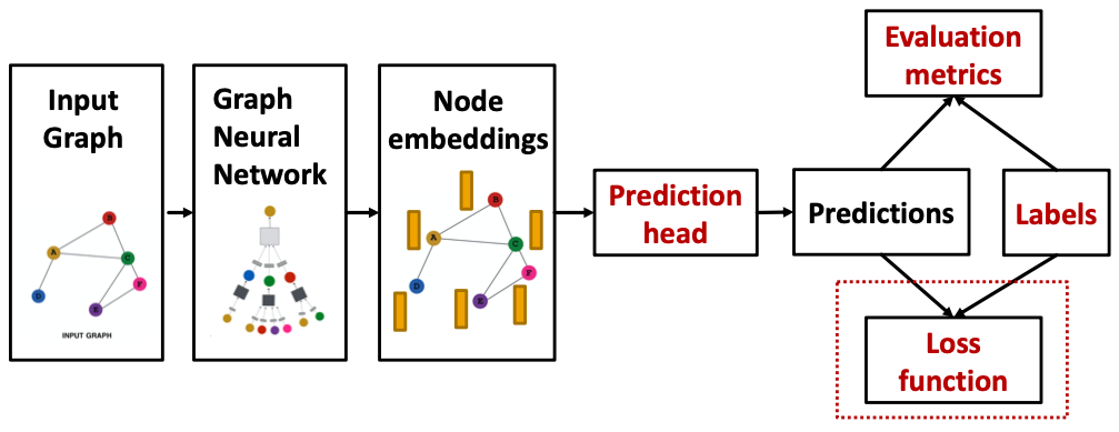
How do we compute the final loss?

Classification loss

Regression loss

Settings for GNN Training

We have $N$ data points

Each data point can be a node/edge/graph

Node-level: prediction $\hat{\text{y}}_v ^{(i)}$ , label $\text{y}_{v}^{(i)}$

Edge-level: prediction $\hat{y}_{uv}^{(i)}$ , label $\text{y}_{uv}^{(i)}$

Graph-level: prediction $\hat{y}_G^{(i)}$ , label $\text{y}_{G}^{(i)}$

Classification: labels $\text{y}^{(i)}$ with discrete value

Regression: labels $\text{y}^{(i)}$ with continuous value

Classification Loss

cross entropy (CE) is a very common loss function in classification

$K$ -way prediction for $i$ -th data point:

\text{CE}(\textbf{y}^{(i)},\hat{\textbf{y}}^{(i)}) = - \sum_{j=1}^K \textbf{y}_j^{(i)} \log(\hat{\textbf{y}}_j^{(i)})

where:

\textbf{y}^{(i)} \in \mathbb{R}^K = \text{one-hot label encoding}]\\ \hat{\textbf{y}^{(i)}} \in \mathbb{R}^K = \text{prediction after} \ \text{Softmax}(\cdot)

Total loss over all $N$ training examples

Regression Loss

For regression tasks we often use Mean Squared Error (MSE) a.k.a $L_2$ loss

$K$ -way regression for data point $(i)$ :

\text{MSE}(y^{(i)},\hat{y}^{(i)}) = \sum_{j=1}^K (y_j^{(i)} - \hat{y}_j^{(i)})^2

where

y^{(i)} \in \mathbb{R}^k = \text{Real valued vector of targets}\\ \hat{\text{y}}^{(i)} \in \mathbb{R}^k = \text{Real valued vecotor of predictions}

Total loss over all $N$ training examplles

\text{Loss} = \sum_{i=1}^N \text{MSE}(y^{(i)},\hat{y}^{(i)})

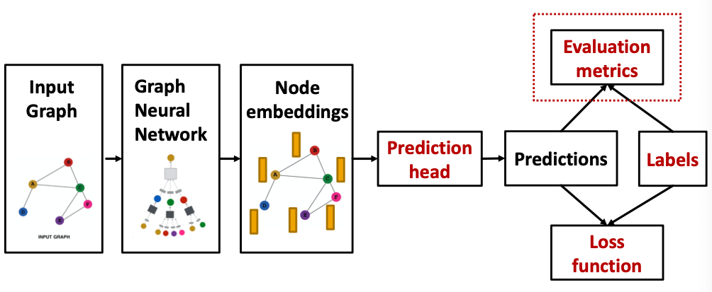
How do we measure the success of a GNN?

Accuracy

ROC AUC

Evaluation Metrics: Regression

Suppose we make predictions for $N$ data points

Root mean square error (RMSE)

\sqrt{\sum_{i=1}^N \frac{(y^{(i)}-\hat{y}^{(i)} )^2}{N}}

Mean absolute error (MAE)

\frac{\sum_{i=1}^N|y^{(i)}-\hat{y}^{(i)}|}{N}

Evaluation Metrics: Classification

Multi-class classification

We simply report the accuracy

\frac{1[argmax(\hat{y}^{(i)}) = y^{(i)}]}{N}

Binary classification
- Metrics sensitive to classification threshold
  - Accuracy
  - Precision / Recall
  - If the range of prediction is $[0,1]$ , we will use $0.5$ as threshold
- Metric Agnostic to classification threshold
  - ROC AUC

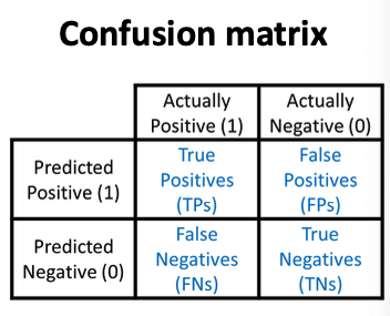
Accuracy

\frac{TP+TN}{TP+TNN+FP+FN} = \frac{TP+TN}{|Dataset|}

Precision (P)

\frac{TP}{TP+FP}

Recall (R)

\frac{TP}{TP+FN}

$F1-$ Score

\frac{2P \times R}{P+R}

ROC Curve: Captures the tradeoff in TPR and FPR as the classification threshold is varied for a binary classifier.

TPR = Recall = \frac{TP}{TP+FN}

FPR = \frac{FP}{FP+TN}

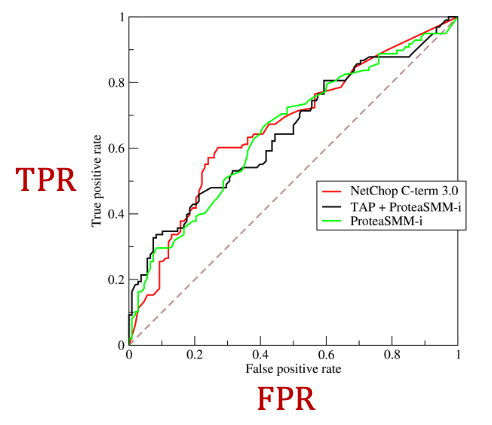
ROC AUC: Area under the ROC Curve.

Intuition: The probability that a classifier will rank a randomly chosen positive instance higher than a randomly chosen negative one.

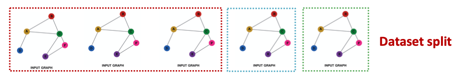
How do we split our dataset into train / validation / test set?

Dataset Split: Fixed / Random Split

Fixed split: we will split our dataset once
- Training set: used for optimizing GNN parameters
- Validation set: develop model / hyperparameters
- Test set: held out until we report final performance

A concern: sometimes we cannot guarantee that the test set will really be held out

Random split: we will randomly split out dataset into training / validation / test
- We report average performance over different random seed.

分割图是特殊的为什么？ Why Splitting Graphs is Special? 或许每个节点都有可能是相互关联的

Suppose we want to split an image dataset?

Image classification: Each data point is an image

Here data points are independent
- Image 5 will not affect our prediction on image 1

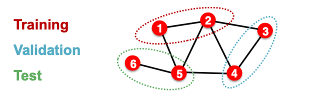
Splitting a graph dataset is different!

Node classification: Each data point is a node

Here data points are NOT independent
- Node 5 will affect our prediction on node 1, because it will participate in message passing $\Longrightarrow$ affect node 1’s embedding

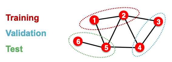
\text{Solution 1 Transductive setting}

The input graph can be observed in all the dataset splits (training, validation and test set)

We will only split the (node) labels
- At training time, we compute embeddings using the entire graph, and train using node 1&2’s labels
- At validation time, we compute embeddings using the entire graph, and evaluate on node 3&4’s labels

\text{Solution 2 Inductive setting}

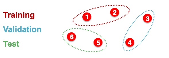
We break the edges between splits to get multiple graphs

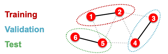
Now we have 3 graphs that are independent. Node 5 will not affect our prediction on node 1 any more.

At training time, we compute embeddings using the graph over node 1&2, and train using node 1&2’s labels

At validation time, we compute embeddings using the graph over node 3&4, and evaluate on node 3&4’s labels

Transductive / Inductive Settings

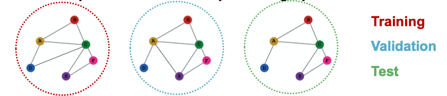
Transductive setting: training / validation / test sets are on the same graph
- The dataset consists of one graph
- The entire graph can be observed in all dataset splits, we only split the labels
- Only applicable to node /edge prediction tasks

Inductive setting: training / validation / test sets are on different graphs
- The dataset consists of multiple graphs
- Each split can only observe the graph within the split. A successful model should generalize to unseen graphs
- Applicable to node /edge / graph tasks

\text{Node Classification}

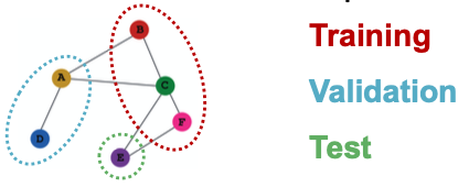
Transductive node classification
- All the splits can observe the entire graph structure, but can only observe the labels of their respective nodes

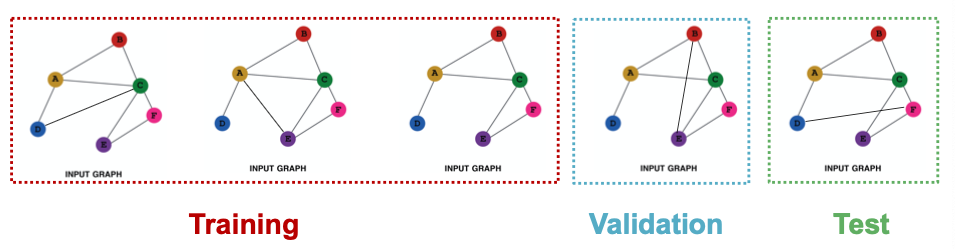
Inductive node classification
- Suppose we have a dataset of 3 graphs
- Each split contains an independent graph

\text{Graph Classification}

Only the inductive setting is well defined for graph classification
- Because we have to test on unseen graphs
- Suppose we have a dataset of 5 graphs. Each split will contain independent graph(s).

\text{Link Prediction}

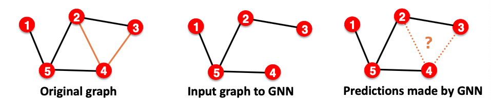
Goal of link prediction: predict missing edges

Setting up link prediction is tricky(确实):
- Link prediction is an unsupervised / self-supervised task. We need to create the labels and dataset splits on our own.
- Concretely, we need to hide some edges from the GNN and the let the GNN predict if the edges exist.

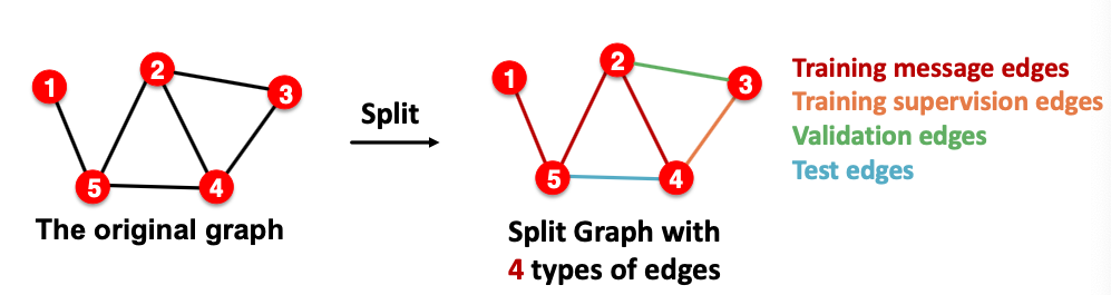
How to set up link prediction?

For link prediction, we will split edges twice

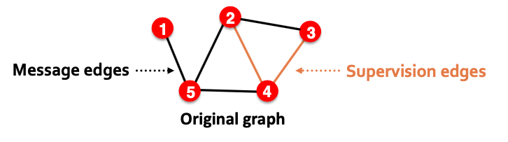
Step 1: Assign 2 types of edges in the original graph
- Message edges: Used for GNN message passing
- Supervision edges: Use for computing objectives
- After step 1:
  - Only message edges will remain in the graph
  - Supervision edges are used as supervision for edge predictions made by the model, will not be fed into GNN!

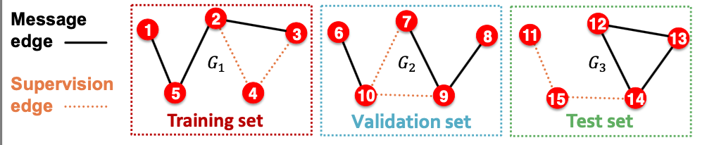
Step 2: Split edges into train / validation / test

Option 1: Inductive link prediction split
- Suppose we have a dataset of 3 graphs. Each inductive split will contain an independent graph.
- In train or val or test set, each graph will have 2 types of edges: message edges + supervision edges
  - Supervision edges are not the input to GNN

Option 2: Transductive link prediction split
- This is default setting when people talk about link prediction
- Suppose we have a dataset of 1 graph
- By definition of “transductive”, the entire graph can be observed in all dataset splits
  - But since edges are both part of graph structure and the supervision, we need to hold out validation / test edges
  - To train the training set, we further need to hold out supervision edges for the training set
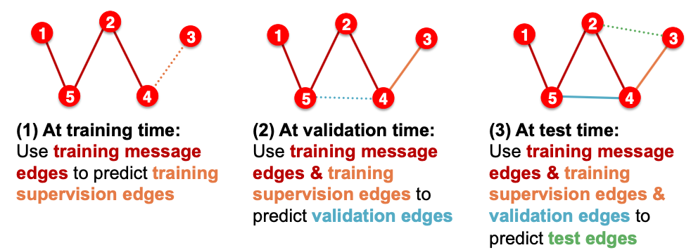
Why do we use growing number of edges?
After training, supervision edges are know to GNN. Therefore, an ideal model should use supervision edges in message passing at validation time. The same applies to the test time.

Summary: Transductive link prediction split
$\text{GNN Training Pipeline}$