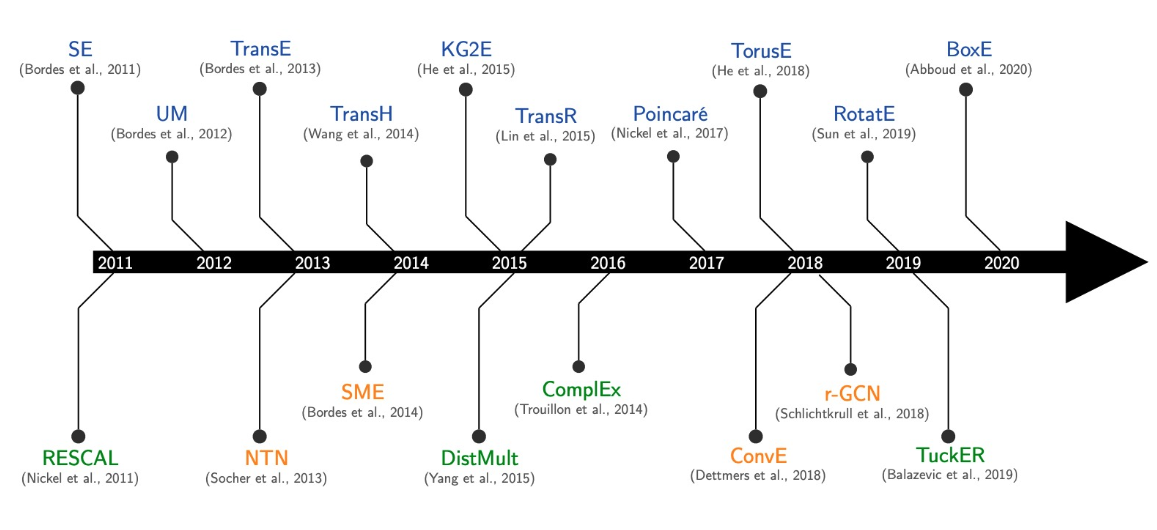
CS224W-Machine Learning with Graph- Knowledge Graph
Knowledge Graph Embeddings
Heterogeneous graphs: a graph with multiple relation types.
Knowledge in graph from: capture entities, types, and relationships
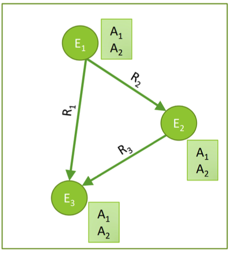
- Nodes are entities.
- Nodes are labeled with their types.
- Edges between two nodes capture relationships between entities.
- Knowledge graph is an example of a heterogeneous graph.
Bibiographic Networks
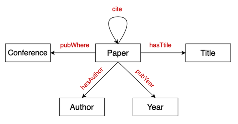
- Node types: paper, title, author, conference, year
- Relation types: pubWhere, pubYear, hasTitle, hasAuthor, cite
Bio Knowledge Graphs
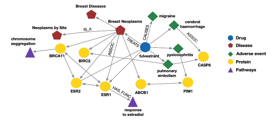
- Node types: drug, disease, adverse event, protein, pathway
- Relation types: has_func, causes, assoc, treats, is_a
Applications of Knowledge Graphs
- Serving information
- Question answering and conversation agents
Knowledge Graph Dataset
- Publicly available KGs:
- FreeBase, Wikidata, Dbpedia, YAGO, NELL, etc.
- Common characteristics:
- Massive: Millions of nodes and edges
- Incomplete: Many. true edges are missing
Knowledge Graph Completion
KG Representation
- Edge in KG are represented as triples
- head has relation with tail
- Key Idea:
- Model entities and relations in embedding space
- Associate entities and relations with shallow embeddings (we do not learn a GNN here!)
- Given a triple , the goal is that the embedding of should be close to the embedding of .
- How to embed ?
- How to define score ?
- Score is high if exists, else is low.
- Model entities and relations in embedding space
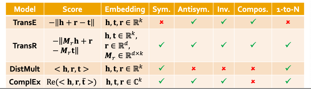
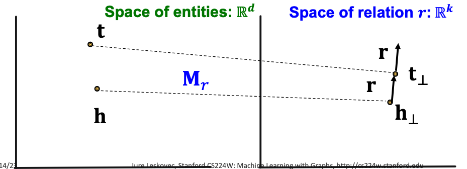
Knowledge Graph Completion: TransE
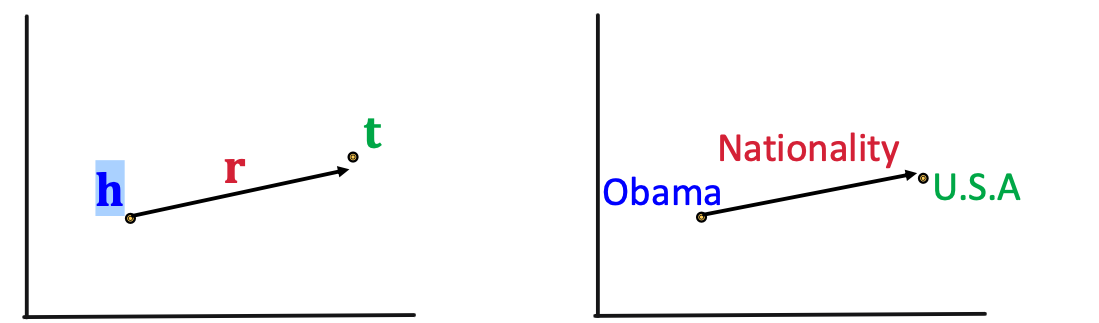
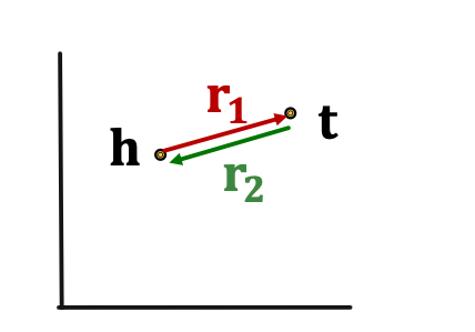
- Intuition: Translation
- For a triple , let be embedding vectors
- TransE: if the given link exists else
- Entity scoring function:
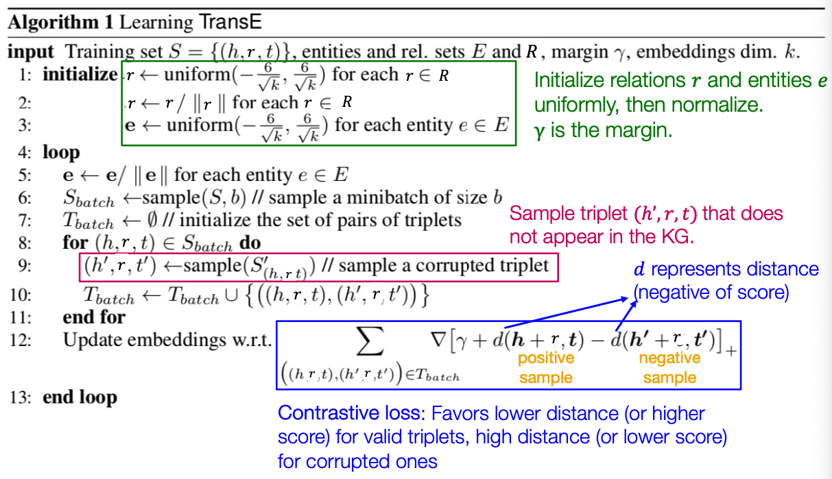
TransE : How to learn?
Relations in a heterogeneous KG have different properties:
- Example:
- Symmetry: If the edge exists in KG, then the edge should also exist.
- Inverse relation: If the edge exists in KG, then the edge should also exist.
Four Relation Patterns
- Symmetric (Antisymmetric) Relation:
- Example:
- Symmetric: Family, Roommate
- Antisymmetric: Hypernym (a word with a broader meaning: poodle vs. dog)
- Example:
- Inverse Relation:
- Example: (Advisor, Advisee)
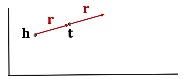
- Composition (Transitive) Relation:
- Example: My mother’s husband is my father
- 1-to-N relations:
- Example: is “StudentsOf”
are all True.
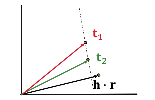
Antisymmetric Relations in TransE
- Antisymmetric Relations:
- Example: Hypernym (a word with a broader meaning: poodle vs. dog)
- TransE can model antisymmetric relations.
- , but
Inverse Relations in TransE
- Inverse Relation:
- Example: (Advisor, Advisee)
- TransE can model inverse relations.
- , we can set
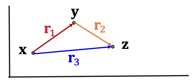
Composition in TransE
- Composition (Transitive) Relation:
- Example: My mother’s husband is my father.
- TransE can mode composition relation.
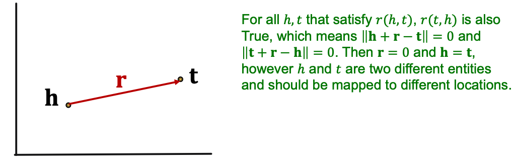
Symmetric Relation: Limitation
- Symmetric Relation:
- Example: Family, Roommate
- TransE cannot model symmetric relations only if
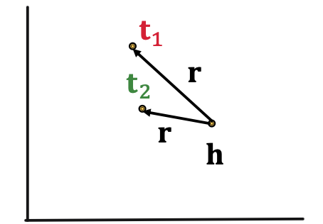
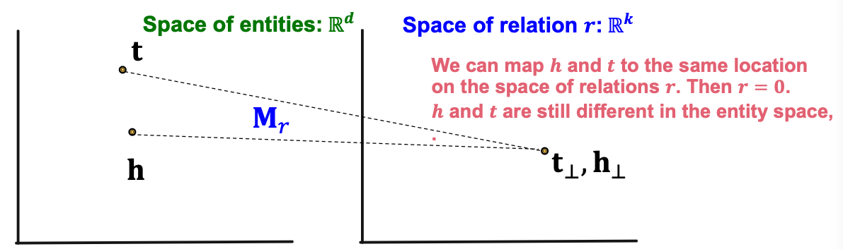
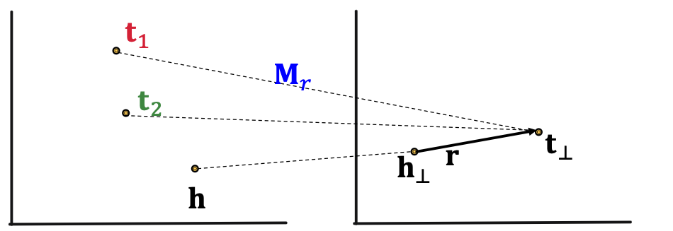
1-to-N Relations: Limitation
- 1-to-N Relations:
- Example: and both exist in the knowledge graph, e.g. is “StudentsOf”
- TransE cannot model 1-to-N relations
- and will map to the same vector, although they are different entities.
-
-
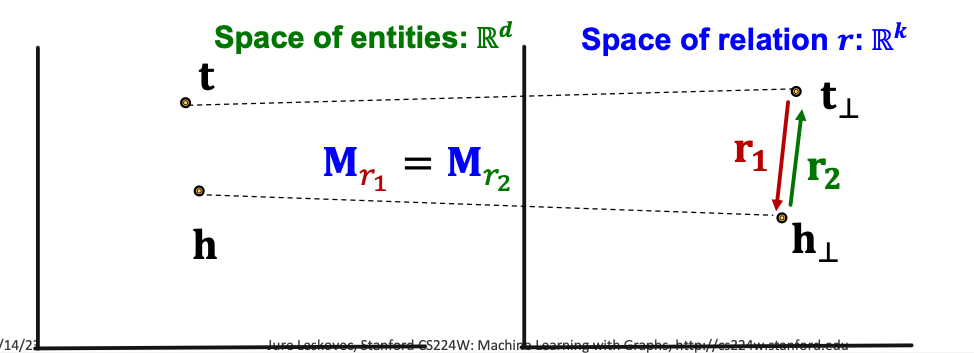
Knowledge Graph Completion: TransR
- TransE models translation of any relation in the same embedding space.
- TransR: model entities as vectors in the entity space and model each relation as vector in relation space with as the projection matrix.
TransR
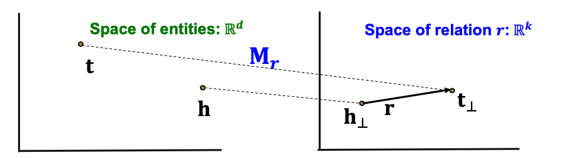
-
- Score function:
Symmetric Relations in TransR
- TransR can model symmetric relations
Antisymmetric Relations in TransR
- TransR can model antisymmetric relations:
1-to-N Relations in TransR
- TransR can model 1-to-N relations
- We can learn so that
- Note that does not need to be equal to !
Inverse Relations in TransR
- TransR can model inverse relations
then
and
Composition Relations in TransR
- TransR can model composition relations.
- TransR models a triple with linear functions. Linear functions are chainable!
- If and are linear, then is also linear:
- Let: then
- If and are linear, then is also linear:
- Background:
- Def: Kernel space of a matrix :
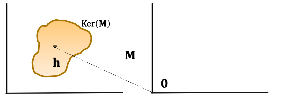
- Assume and
- For
- Same for
- Then, we have
- Construct s.t.
- Since:
-
- has the same shape as
we know exists!
- Set
- We have
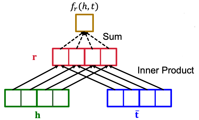
Knowledge Graph Completion: DistMult
New Idea: Bilinear Modeling
- So far: The scoring function is negative of distance in TransE and TransR
- Idea: Use bilinear modeling: Score function
- Problem: Too general and prone to overfitting
- Matrix A is too expressive
- Fix: Limit A to be diagonal
- This is called DistMult
- Problem: Too general and prone to overfitting
New Idea: Bilinear Modeling
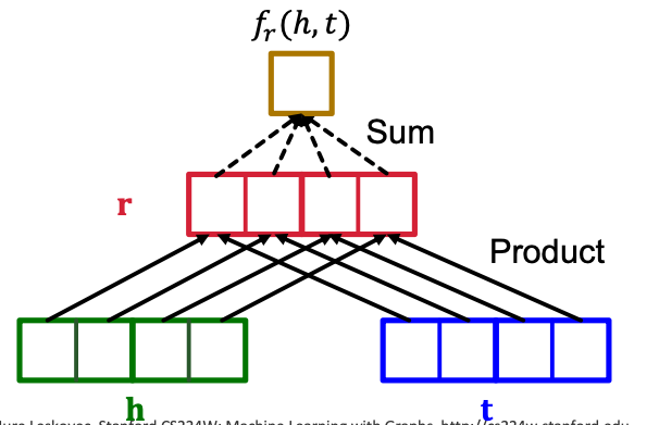
- DistMult: Entities & relations are vectors in
- Score function:
-
- Can be viewed as a cosine similarity between and , where is defined as
- Example:
1-to-N Relations in DistMult
- 1-to-N Relation:
- If and exist in the knowledge graph
- DistMult can model 1-to-N relations
Symmetric Relations in DistMult
- DistMult can naturally model symmetric relations
- Due to the commutative property of multiplication
Limitation: Antisymmetric Relations
- DisMult can not model antisymmetric relations
- and always have same score!
Limitation: Inverse Relations
- DistMult can not model inverse relations
- Assume DistMult does model inverse relations:
- For example, solves this
- But semantically this does not make sense: The embedding of “Advisor” relation should not be the same as “Advisee” relation.
Limitation: Composition Relations
- DistMult can not model composition of relations
- Because dot product is commutative DisMult does not distinguish between head and tail entities, so it cannot model composition.
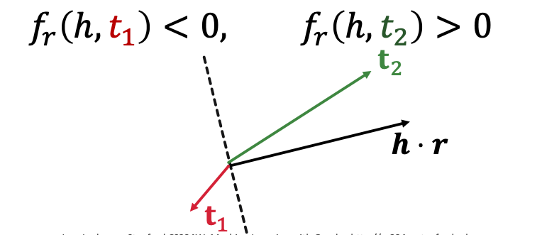
Knowledge Graph Completion: ComplEx
- Based on DistMult, ComplEx embeds entities and relations in Complex vector space
- ComplEx: model entities and relations using vector in
- Score function
Antisymmetric Relations in ComplEx
- ComplEx can model antisymmetric relations
- The model is expressive enough to learn
- High
- Low
Due to the asymmetric modeling using complex conjugate
- The model is expressive enough to learn
Symmetric Relations in ComplEx
- ComplEx can model symmetric relations
- When , we have
Inverser Relations in ComplEX
- ComplEx can model inverse relations
-
- ComplEx conjugate of
- is exactly
-
Composition and 1-to-N in ComplEx
- ComplEx share the same property with DistMult
- Can not model composition relations
- Can model 1-to-N relations